

The K Nearest Neighbors Algorithm often called as K-NN, is a supervised learning algorithm which can be used for both, classification and regression. In both the cases, however, the input is same
– K closest training points.
In K-NN classification, the test data point is assigned to the class of the majority of its K nearest training points, which are also called its K nearest neighbors. In the case of K-NN regression, the output value for a test data point is typically the average of the values of its K nearest neighbors.
In this article, first, we will explain the 1 Nearest Neighbor algorithm, which is essentially the K-NN algorithm with K=1. After that, we will explain the actual K-NN algorithm.
1 – Nearest Neighbor Regression
Consider the following relationship between features (denoted by x) and target values, often called as ‘classes’ (denoted by y):
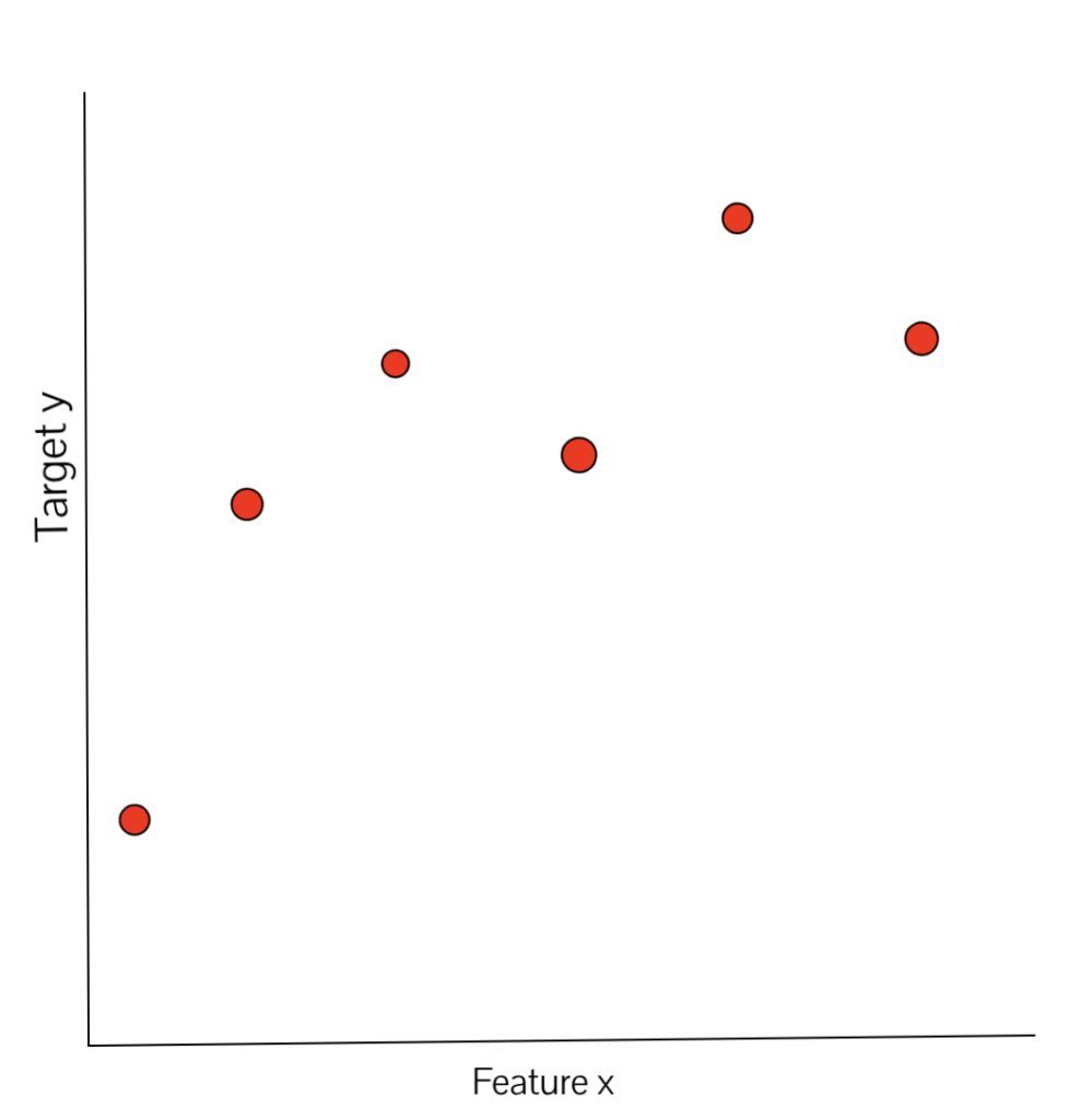
In the points plotted above, each xi has a corresponding yi. In K-NN regression, the output value for a new test data point is equal to the average of the target values of its K nearest neighbors. Since we are studying the case of 1-NN, the output value for a new test data point will be equal to the target value of its nearest neighbor. Hence, the 1-NN regression plot for the above-mentioned case will look similar to the figure below:
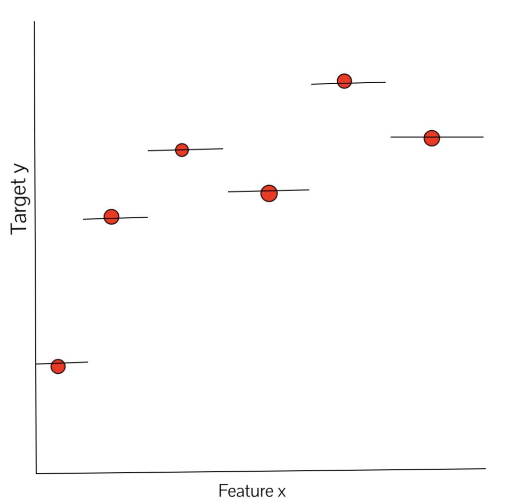
The horizontal line going through a given training data point above shows the range of values of x for which the target value will be same as that of the given training data point. Hence, if a new test data point, xa is introduced, and it is nearest to the training data point xi (whose target value is yi), the output target value of the point xa will be equal to yi. Notice that as a regression, this predictor function is locally constant; since as we move slightly, we continue to have the same nearest neighbor, which leads to the prediction of the same target value.
Please note that a point that is equidistant from any 2 given points lies on the perpendicular bisector of the line joining the 2 points. The horizontal lines on the data points in the above plot are generated using the same principle.
1 – Nearest Neighbor Classification
In the classification K-NN problem, the target values are discrete and for a new test data point, its output target value is equal to the target value of the majority of the K nearest training points. If the value of K is odd, there will not be any ties. Hence, the output target value will be equal to the target value of one of the existing training points.
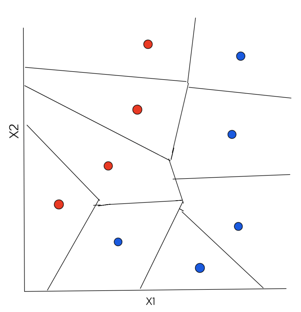
Consider the figure below. It has data points which belong to one of the 2 classes (target values): 1 (denoted by red color) and 2 (denoted by blue color). Each data point consists of 2 features – X1 and X2.
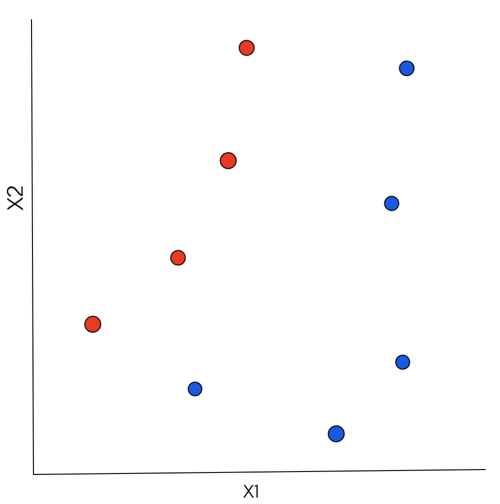
For a newly introduced test data point, its Euclidean distance is computed from each training data point to find the nearest neighbor. The formula for the Euclidean distance between 2 points x and x’ is:
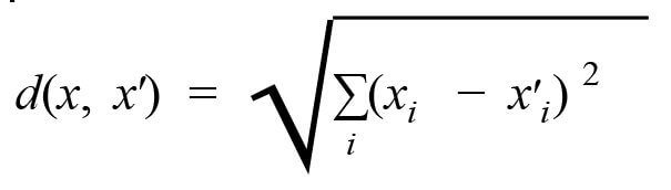
The output target value for the test data point is equal to the target value of the training data point that is nearest to the test data point.
If we evaluate the Euclidean distance for every possible point X, a function can be defined – all the points X that are closest to the points with target value 1 (red) will have output target value as 1 and all the points X that are closest to the points with target value 2 (blue) will have target output value of 2. Between them, there will be an abrupt change, known as the Decision Boundary. The decision boundary is formed by the set of points, both sides of which there are data points of different classes or target values.
Just like in the case of 1-NN regression, it’s clear that there will be a region around each training data point where any new test data point will be closest to that training data point. This is what we call as Voronoi Tessellation – each datum is assigned to a region, in which all points are closer to it than any other datum. All the test data points that lie in the region of a particular training data point will have the output target value equal to the target value of that training data point.
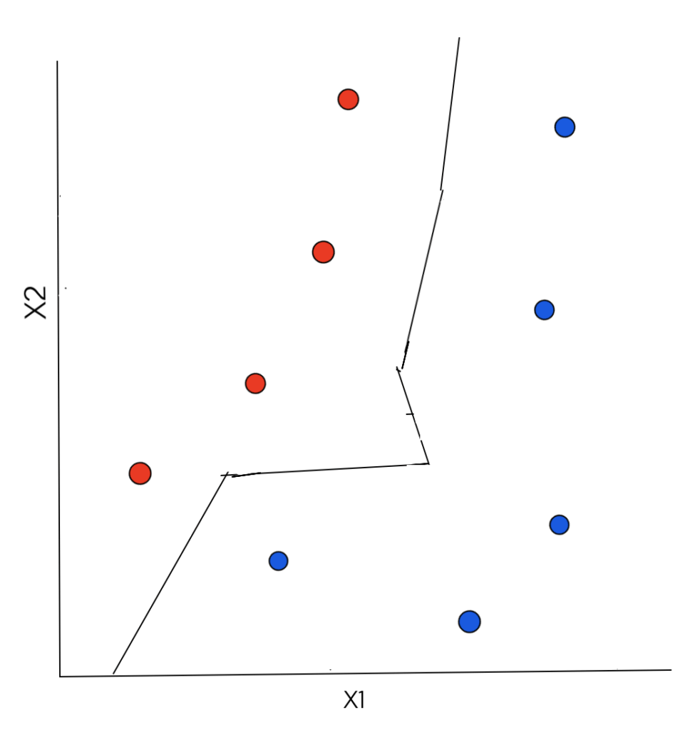
The final decision boundary that separates the 2 classes from one another is piecewise linear and is shown below:
K.N earest Neighbor Classification
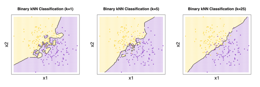
The K-NN algorithm produces piecewise linear decision boundary. As the value of K increases, the decision boundary becomes even simpler. This is because with the increase in the value of K, the overfitting of the model decreases and it becomes more generalized. In majority voting, there is less emphasis on individual points, which leads to simplification of the decision boundary.
The figures below will help you visualize the same:
Error Rates vs K
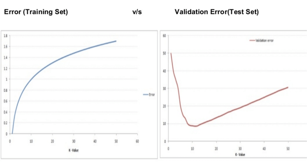
When K=1, each data point has a region present around it that predicts the target value of that data point. Each training data point is predicted correctly since the model memorizes the target value of all the data points in the training set. Such a model is highly overfitted. In case of a large value of K, this is not true. The value of some data points may be predicted wrong. Hence initially, with increasing K, the error on training data increases. However, after a certain value of K, the error on the training data remains almost constant.
The graph of the error on test data is of a completely different shape. When K=1, the error on test data is high. It decreases as K increases. After a certain value of K, the error on the test data increases again. Hence, the ideal value of K is where the error on test data is minimum.
The figure below shows the error on the training dataset and the test dataset:
Pseudo Code of K-NN
The K-NN model can be implemented by following the steps mentioned below:
1. Load the training dataset
2. Initialize the value of K
3. To get the predicted class of a particular test data point, iterate over all data points in the training dataset
a. Find the distance of the test data point from each of the training data points.
4. Sort the distances calculated in the above step in ascending order.
5. Get the top K training data points that are nearest to the test data point.
6. Find the most frequently occurring target value among these training data points.
7. Return the predicted value, which is the one found in the above step.
K-NN algorithm is one of the simplest machine learning algorithms. It takes less time for computation and also provides competitive results. It is often used in statistical estimation and pattern recognition.

