

Order of the New World.
Personalization & Automation.
These two words describe where the world is headed. And I don’t think you’ll disagree if we say that this accelerated paradigm shift is more so because of the rise of Artificial Intelligence technologies than any other.
This shift is fuelled by 2.5 quintillion bytes of data injected into this rocket each day and companies are only getting creative. Today, you try to search for a holiday destination on the Internet, and by the time you finish, companies in the travel business already have spammed your mail with offers and personalized discounts.
Artificial Intelligence Technologies are getting increasingly dominant and accurate with anticipating what the end-user wants. But this is the news of 2016, of course. You know it, we know it. Done and dusted. What’s up now?
Well, post-2016, they’ve taken a significant step further and we’ve seen the steady rise of what’s been largely called the Emotional AI Technology.
We’ve said the world pulses out 2.5 quintillion bytes of data each day. This data is in the form of web searches, social media interactions, images, videos etc, but here’s a thought before you go further.
What about the data that isn’t being captured?
The travel companies know somebody is trying to get a good deal on her flight to Toronto through her web searches, but what about the way in which she reacts to a particular piece of clothing in a store?
Well, you’ve guessed it. Welcome to 2019.
Let us walk you through an example quick:
Emotion AI systems, like any other system, are made of two components. Hardware and Software. The hardware component involves small cameras or sensors, deployed in stores in high-traffic locations, such as shelves, aisle end caps, checkout lines, and entrances and exits — anywhere and at any stage in the shopping process where retailers and brands are most interested in gauging shopper sentiment. The system records the facial expressions of individual shoppers, and the computer vision, AI and analytics components recognize, classify and interpret the emotions they appear to be expressed at a given moment.
The result could be a compilation of various emotional responses retailers and brands could access to help them make decisions about important factors that may fuel the buying decision, such as:
- Product pricing, packaging and branding: If emotional responses skew negative, it might be time to lower prices. If shoppers examine packages and appear confused, it might be time for a redesign.
- Inventory availability and replenishment: If shoppers appear happy about certain flavors, perhaps stock more of those, less of the flavours they frown at and push aside.
- Shelf placement, store and aisle layouts: If emotional responses suggest frustration, perhaps a reconfiguration of product displays or a move to a different aisle is in order.
But hey, what’s music got to do with any of this?
AI Redefines Genres.
Consider this.
There are more than 25,000 new tracks uploaded to Spotify every day and AI is critical for helping sort through the options and delivering recommendations to listeners based on what they’ve listened to in the past.
Spotify heavily leverages AI to deliver the most personalized experience possible to its users in the form of customized curated playlists updated weekly. The impact of this is that AI has redefined the term “music genre” because AI-generated playlists are made not based on genre, but what is determined to be good music keeping the user in mind all through which falls under the realm of Emotional AI. In fact, there might come a time where genres become completely obsolete together and Spotify’s playlists (Hype, Beast etc) become what we increasingly recognize music better by.
In addition to this, our current paradigm of infinite choice is broken and recommends a new model of trusted recommendations as in the case of already hugely successful Netflix.
Google’s Magenta project, an open-source platform, produced songs written and performed by AI and Sony developed Flow Machines, an AI system that’s already released “Daddy’s Car,” a song created by AI. Not to mention, AI Music Synthesis algorithms. Composers openly admit to going to AI for initial compositional ideas to develop their music from. Automising entire musical instruments during live playback is being experimented with. The impact of AI in the music industry internationally is growing leaps and bounds and all of it is under the realm of Emotional AI.
Pre-processing Music Using Python
With the backdrop of Emotional AI, it’s impact and what’s bleeding edge in the Music AI industry, let’s being our deep dive into pre-processing music in Python.
Libraries
There are a vast number of libraries available for music processing in Python. But the most well documented, and also having the most versatile functionality out of all others, in our experience, is Librosa.
Installing Librosa is easy:
pip install librosa
or
conda install -c conda-forge librosa (If using Anaconda)
When working on any project, you will always want to visualize the data you are working on. However, the catch with music specifically is that visualization often does not help analysis.
Let’s understand why with an example.
We’ll assume we’re working on genre classification problem where our Machine Learning model wants to accept a song as input and classify its genre as output.
Let’s start with a music file, say, Clarity by John Mayer. You can download this sample music file here:
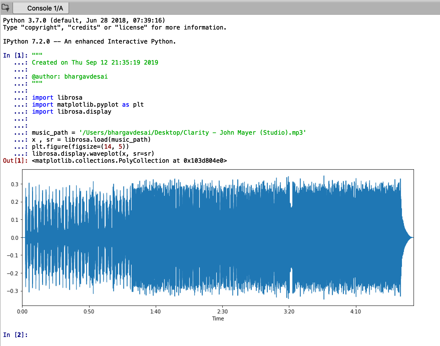
Here’s what you do to visualize music (or audio segments in general) in librosa:
import librosa
import matplotlib.pyplot as plt
import librosa.display

music_path = '/Users/bhargavdesai/Desktop/Clarity - John Mayer (Studio).mp3'
x , sr = librosa.load(music_path)
plt.figure(figsize=(14, 5))
librosa.display.waveplot(x, sr=sr)
The output for the following piece of code is put down below. The problem is apparent. It is hard to understand what we might gain from visualizing the entire music file. To make matters worse, as an exercise you can try visualizing other music files, they will look almost the same to this plot that we have here.
So what do we do?
At Eduonix, we believe in looking at things in the right way to understand the fundamentals. So first, let’s start with the basics and answer the question, “What is music?”, and then take a little bit of guidance from the one thing that we know for sure gives a very clear picture of any sound to our brain: the cochlea.
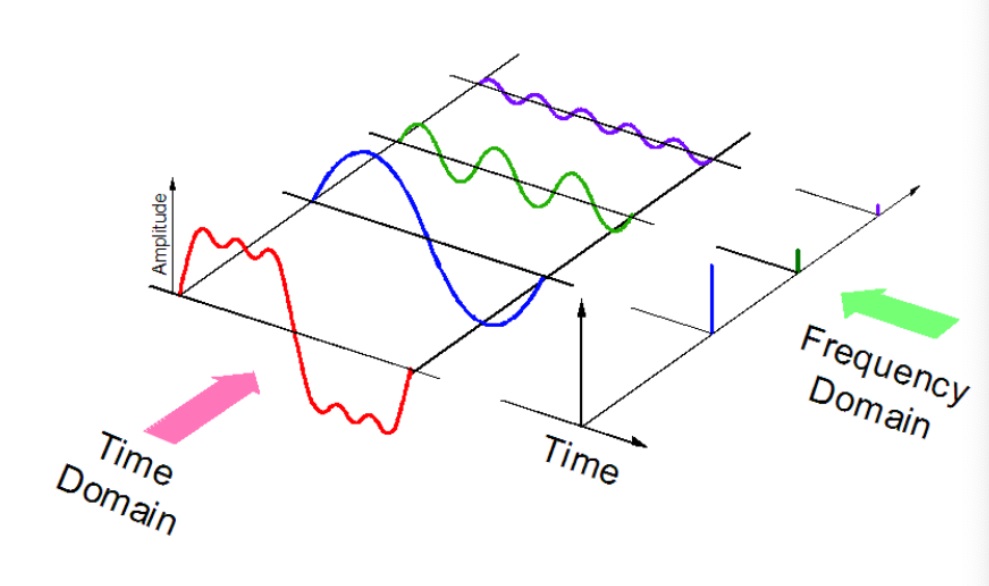
Well, music is nothing but a harmonious mix of frequencies and the cochlea in our ear is nothing but a frequency sensitive tube that distills any incoming sound into constituent frequencies which is then relayed to the brain using the auditory nerve.
Let’s clear that up with a small graphic. Assume the red signal is a small music signal out of a complete song. The blue, green and violet decomposition is exactly what our cochlea does to that music signal and this mix of harmonics or frequencies is what determines whether we like the music, or we don’t.
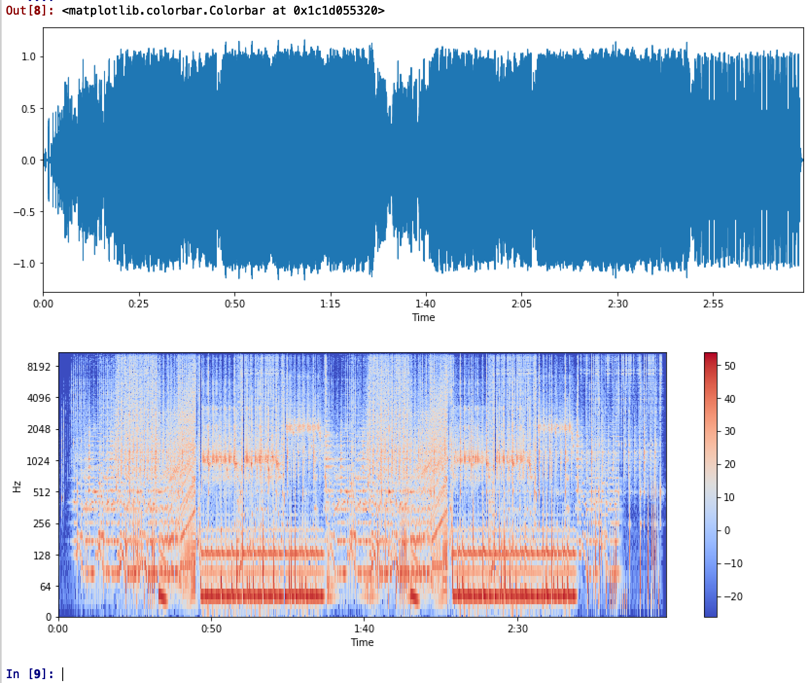
Let’s try this in code, shall we? We’ll try to break the song into its constituent frequencies and plot it. The resulting plot is often called the spectrogram since we’re decomposing the song into its ‘spectrum of frequencies’
frequencies = librosa.stft(x)
freq_to_dB = librosa.amplitude_to_db(abs(frequencies))
plt.figure(figsize=(14, 5))
librosa.display.specshow(freq_to_dB, sr=sr, x_axis='time', y_axis='hz')
plt.colorbar()
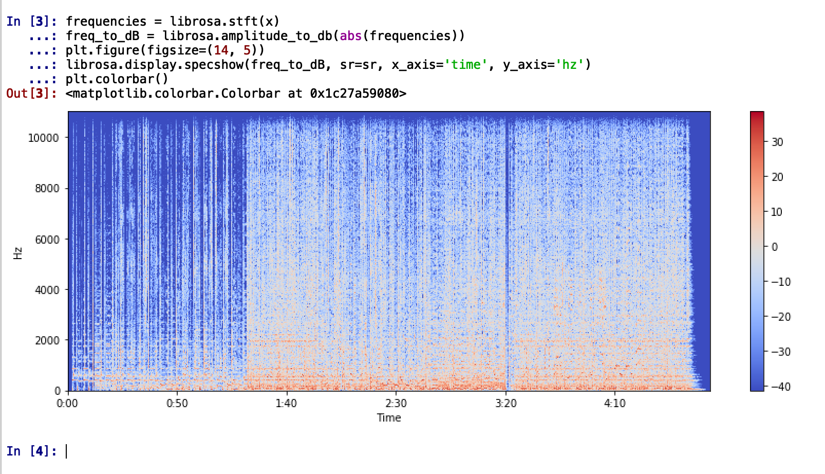
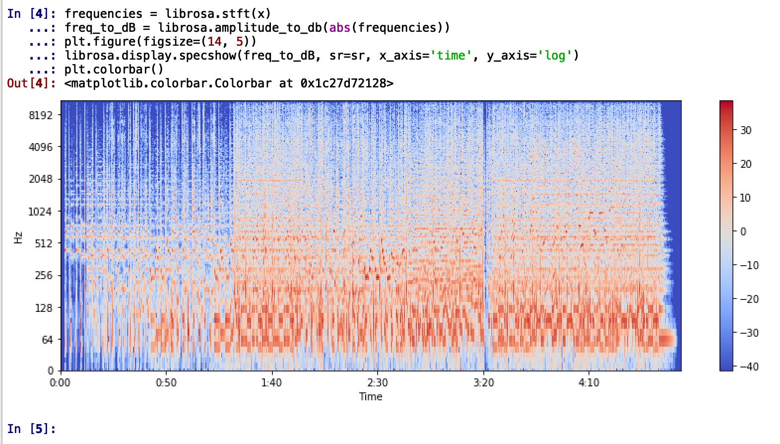
It is better to use a log scale to represent the frequency since it is clear that the song has a lot of low-frequency sounds. (Change y_axis parameter to y_axis=‘log’)
Immediately, we can tell that the song the dominant frequencies of the song are between the range of 20Hz to 256KHz with some extending up to 512KHz. This tells us that the song is likely to be mellow with bass, drums, percussive elements and low octave trumpets which is indeed the case.
We’ll take another example with another song that will make the intuition clear for using a spectrogram. Here’s the song we’ll be using next:
Following the same code, just passing a different file path of our song file, here’s what we have:
As promised, with just the plot of the song, there is really strong to infer. But if we look at the spectrogram, we see some really low bass with a repetitive pattern and the dominant frequency range of up to more than 2KHz. Any guesses about the genre of people?
Yes indeed! That’s EDM! And the song is Animals by Martin Garrix.
The power of the spectrogram becomes clearly obvious here. We could easily tell without any heavy experience in music that the genre of this song is EDM.
Consequently, for any genre classification problem, instead of passing the raw music file, we could use a Convolutional Neural Network on the spectrograms to derive ‘features’ from the plot (like how we picked out dominant low bass with a repetitive pattern meant EDM, but more abstract and complex ones) to classify genre.
Deriving More Features
Usually, a spectrogram is a sufficient enough feature for tasks like genre classification or music recommendation, but it might not always be possible to use a spectrogram because a Convolutional Neural Network can take some time train (although with GPU instances available that’s not such a big problem anymore) and you want to use a Deep Neural Network instead or maybe you want supplementary features along with the spectrogram to increase the prediction accuracy of your model.
We’ve got you covered.
Let’s look at some more possible pre-processing that you can do with music in Python:
Zero-Crossing Rate
Zero-Crossing Rate or ZCR is exactly what it says it is. It is the rate at which the signal crosses the ‘zero’ amplitude line. That is the number of changes from positive to negative or back. ZCR is usually higher for highly percussive sounds. Calculating it is simple enough with librosa.
zero_crossings = librosa.zero_crossings(x, pad=False)
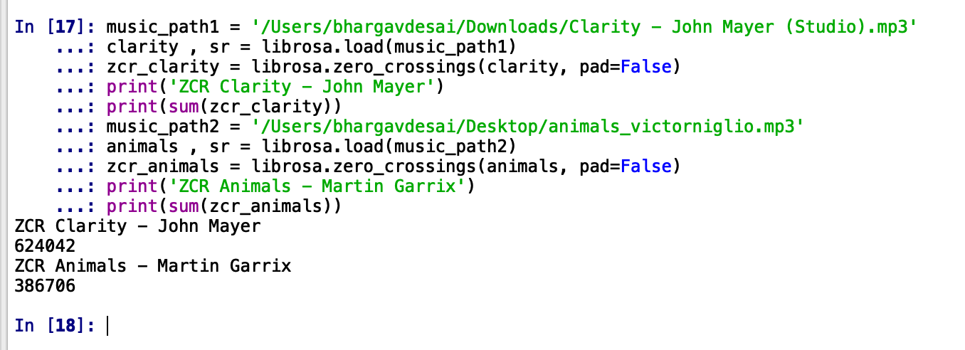
We’ll pass both our previous songs, Clarity – John Mayer and Animals – Martin Garrix to this function and see the difference in ZCR. We expect the ZCR for Clarity to be greater because of the percussive element in Clarity.
As we expected. ZCR for Clarity is significantly more than for Animals. It seems like ZXR is a feature our classifier would love to make use of for its keen eye for percussion-like those in metal and rock.
Spectral Centroid
Spectral Centroid, again as the name suggests, indicates where the ”centre of mass” for a sound is located and is calculated as the weighted mean of the frequencies present in the sound. Consider two songs, one from a blues genre and the other belonging to metal. Now as compared to the blues genre song which is the same throughout its length, the metal song has more frequencies towards the end. So spectral centroid for blues song will lie somewhere near the middle of its spectrum while that for a metal song would be towards its end. The code for Spectral Centroid is again, simple.
spectral_centroids = librosa.feature.spectral_centroid(x, sr=sr)[0]
Mel Frequency Cepstral Coefficients (MFCCs)
The Mel frequency cepstral coefficients (MFCCs) of a signal are a small set of features (usually about 13-20) which concisely describe the overall shape of the spectral envelope. If the shape of the envelope can be determined or captured, any song can be reconstructed. This means MFCCs can be used along with other spectral features to very accurately determine each song. Consequently, our classifier would find heavy use for MFCCs.
MFCCs can be calculated by:
mfccs = librosa.feature.mfcc(x, sr=sr)
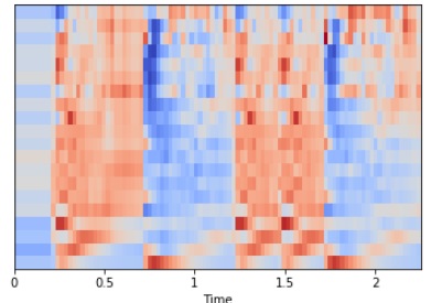
We can display the MFCCs but usually, they have no easy interpretation for a human as can be seen from the plot and so correspondingly it is not suggested to use MFCCs plots for Convolutional Neural Networks classifications over Spectrogram plots.
librosa.display.specshow(mfccs, sr=sr, x_axis=‘time')
A full-fledged tutorial on music genre classification is beyond the scope of this blog and if requested, will be covered in detail later using Convolutional Neural Networks and Deep Neural Networks along with a music recommendation using Deep Learning tutorial.
Until then, we hope you found these pre-processing tips useful!

