

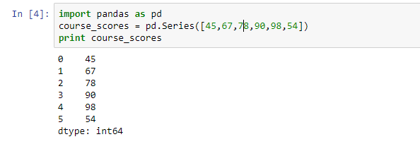
The foundation of Pandas is the Series and DataFrame data structures. Although these objects do not solve every data problem they are an excellent solution for frequently encountered problems. The Series data structure is a one-dimensional object holding a NumPy array and an index. There are different ways in which a Series object can be created. One approach is using a Python list as shown below. When the series is printed, the first column shows the index while the second column shows the actual data.
import pandas as pd

course_scores = pd.Series([45,67,78,90,98,54])

print course_scores
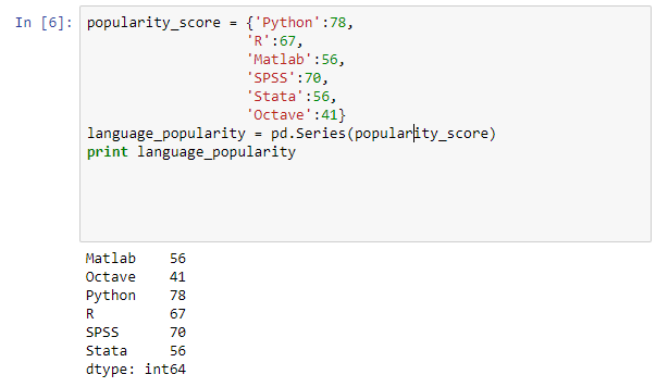
Another approach that can be used to create a Series object is using a Python dictionary as shown below. When using a dictionary to create a Series object the keys will become the Series index.
popularity_score = {'Python':78,
                   'R':67,
                   'Matlab':56,
                   'SPSS':70,
                   'Stata':56,
                   'Octave':41}
language_popularity = pd.Series(popularity_score)
print language_popularity
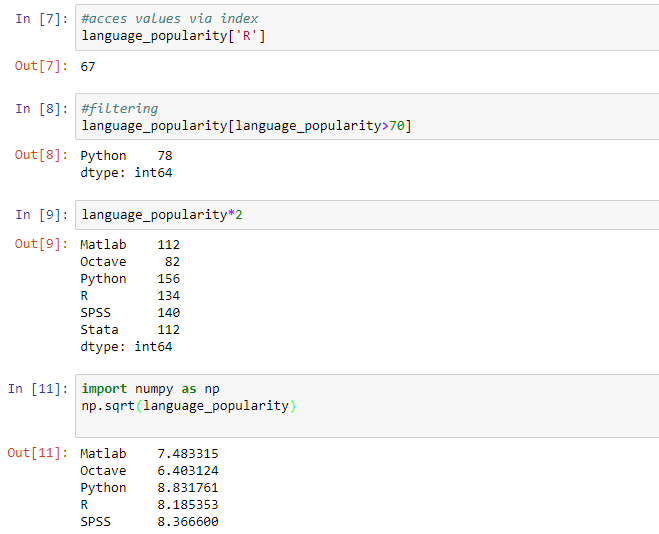
Just like Numpy arrays selecting values via an index, filtering, scalar multiplication and mathematical functions are supported. Examples of these operations are shown below.
#acces values via index

language_popularity['R']

#filtering

language_popularity[language_popularity>70]

#mathematical operations

language_popularity*2

import numpy as np

np.sqrt(language_popularity)
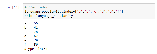
After a Series object has been created you can easily change an index by assigning a new index.
#alter index

language_popularity.index=['a','b','c','d','e','f']

print language_popularity
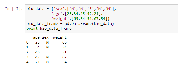
A DataFrame has a tabular structure similar to the one used on spreadsheets. There are multiple named columns holding different data types. When a column has different data types a type that can accommodate all of them will be selected. There are different ways of creating DataFrames. A frequently used approach is passing Numpy arrays or lists that must be of equal length to the DataFrame constructor. An example is shown below.
bio_data = {'sex':['M','M','F','M','M'],

           'age':[23,34,45,42,21],

           'weight':[65,54,51,67,54]}

bio_data_frame = pd.DataFrame(bio_data)

print bio_data_frame
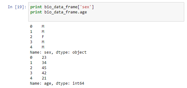
A column in the data frame can be accessed by using the column name as an ‘index’ or by accessing the attributes of the data frame.
print bio_data_frame['sex']

print bio_data_frame.age
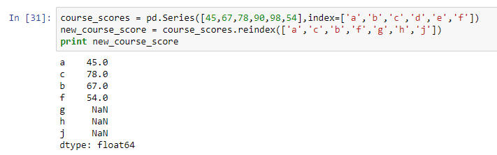
After creating a pandas object there are different manipulations that can be done on the object. When you need your data to adapt to a new index you call the reindex method. This method will rearrange your data and create missing values on new index values.
course_scores = pd.Series([45,67,78,90,98,54],index=['a','b','c','d','e','f'])

new_course_score = course_scores.reindex(['a','c','b','f','g','h','j'])

print new_course_score
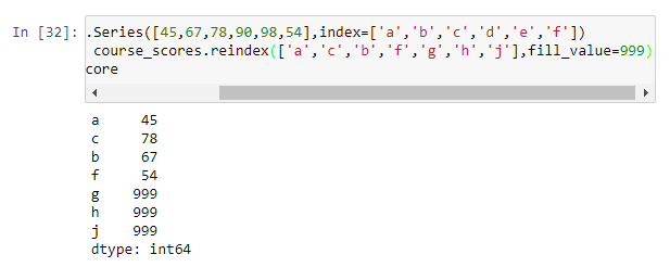
To avoid missing values being introduced after reindexing you specify an alternative value.
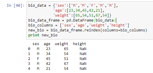
When working with a data frame reindex enables you to alter the columns and rows. Altering rows is done just like in a Series object. An example of altering columns is shown below.
bio_data = {'sex':['M','M','F','M','M'],

           'age':[23,34,45,42,21],

           'weight':[65,54,51,67,54]}

bio_data_frame = pd.DataFrame(bio_data)

bio_columns = ['sex','age','weight','height']

new_bio = bio_data_frame.reindex(columns=bio_columns)

print new_bio
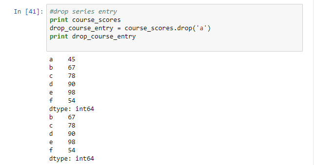
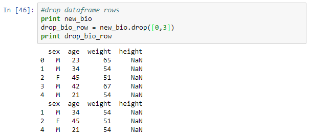
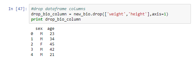
When you need to remove a specific value from a Series or DataFrame you just need to pass an index. In a DataFrame you can delete a row or a column. Examples are shown below.
#drop series entry

print course_scores

drop_course_entry = course_scores.drop('a')

print drop_course_entry
 #drop dataframe rows

print new_bio

drop_bio_row = new_bio.drop([0,3])

print drop_bio_row
#drop dataframe columns

drop_bio_column = new_bio.drop(['weight','height'],axis=1)

print drop_bio_column
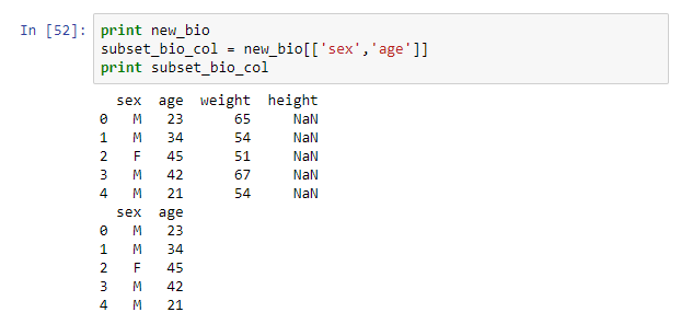
A pandas DataFrame offers different ways of indexing and selection rows and columns. To select one or several columns the notation below is used.
print new_bio

subset_bio_col = new_bio[['sex','age']]

print subset_bio_col
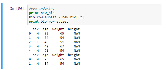
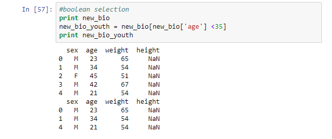
Rows in a DataFrame can be selected by indexing or by Boolean comparison. Examples are shown below.
#row indexing

print new_bio

bio_row_subset = new_bio[:2]

print bio_row_subset
#boolean selection

print new_bio

new_bio_youth = new_bio[new_bio['age'] <35]

print new_bio_youth
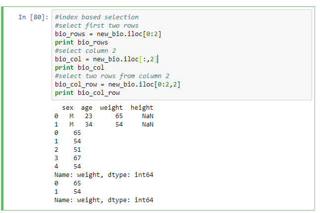
To select a subset of rows and columns iloc and loc indexing are used. To select rows and columns based on labels you use loc while to do selection based on integer index you use iloc. Selection of a single row using iloc will return a Series object while the selection of multiple rows or a complete column will return a DataFrame. These selection approaches require you specify the row and a column selector. Examples are shown below.
#index based selection

#select first two rows

bio_rows = new_bio.iloc[0:2]

print bio_rows

#select column 2

bio_col = new_bio.iloc[:,2]

print bio_col

#select two rows from column 2

bio_col_row = new_bio.iloc[0:2,2]

print bio_col_row
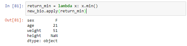
To implement element-wise operations to each column or row of a DataFrame the apply method is used. For example to return the lowest value in each column the syntax below is used.
return_min = lambda x: x.min()

new_bio.apply(return_min)
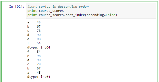
To support data sorting the sort_index method can be used on a Series or DataFrame object. DataFrame objects can be sorted on either axis. To sort by the values of a Series the order method is available. When you need to sort by one or more columns you pass column names to by option. Examples are shown below.
#sort series in descending order

print course_scores

print course_scores.sort_index(ascending=False)
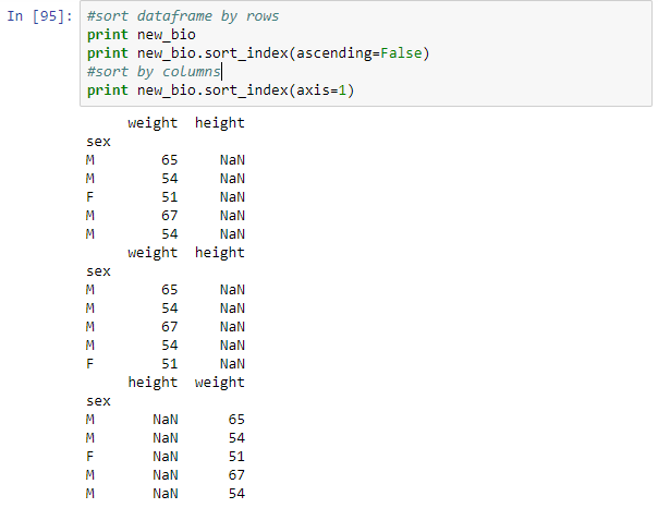
#sort dataframe by rows

print new_bio

print new_bio.sort_index(ascending=False)

#sort by columns

print new_bio.sort_index(axis=1)
Methods to produce descriptive statistics are built into Pandas objects and this provides a simple and efficient way of summarizing data. Some commonly used methods are discussed below.
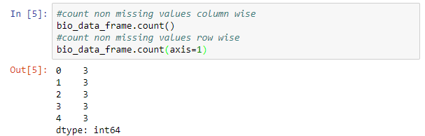
The count method returns the number of non-missing values row wise or column wise. An example is shown below.
#count non missing values column wise

bio_data_frame.count()

#count non missing values row wise

bio_data_frame.count(axis=1)
To get the minimum and maximum values the methods min and max are used. To get the lowest and highest index values the methods idxmin and idxmax are used. To get sample quantile the method quantile is used. To get the mean, median or sum of values the methods mean, median and sum are used. Variance is obtained using the method var, the standard deviation is obtained using the method std, while skewness and kurtosis are obtained using the methods skew and kurt.
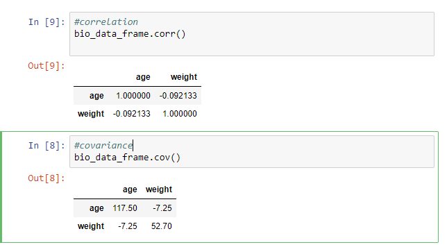
The correlation and covariance are pairwise computations and they are obtained using the methods corr and cov.
#correlation

bio_data_frame.corr()

#covariance

bio_data_frame.cov()
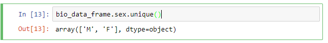
To check for duplicates in a column the unique method is used. For example to check if the sex column has only M and F values.
bio_data_frame.sex.unique()
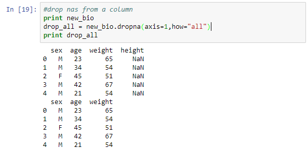
In practice, most data sets will have missing values. It is prudent to investigate the reason for missing values before taking any action. There are different ways of handling missing values built into pandas objects. To remove known missing values the method dropna is used. Dropping missing values is a bit trick in DataFrames. The default behavior is dropna filters out all rows with missing values. To delete columns you need to specify the axis.
#drop nas from a column

print new_bio

drop_all = new_bio.dropna(axis=1,how="all")

print drop_all
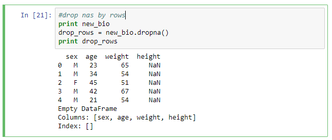
#drop nas by rows

print new_bio

drop_rows = new_bio.dropna()

print drop_rows
This tutorial covered frequently used data manipulation techniques in pandas. Concepts covered were creating pandas objects, reindexing, selecting rows and columns, applying functions, sorting data, summarizing data and handling missing values.
In the meantime, now you can learn Data Science and Analysis: Make DataFrames in Padas and Python.

