Linear Discriminant Analysis With Scikit-Learn

Introduction

Principal Component Analysis (PCA) and Linear Discriminant Analysis (LDA) are well-known dimensionality reduction techniques, which are especially useful when working with sparsely populated structured big data, or when features in a vector space are not linearly dependent. [A vector has a linearly dependent dimension if said dimension can be represented as a linear combination of one or more other dimensions.] Thus, PCA is an unsupervised algorithm for dimensionality reduction, whereas LDA is a supervised algorithm which finds a subspace that maximizes the separation between features.

The advantage that LDA offers is that it works as a separator for classes, that is, as a classifier. However, LDA can become prone to overfitting and is vulnerable to noise/outliers.

In the Scikit-Learn Documentation, the LDA module is defined as “A classifier with a linear decision boundary, generated by fitting class conditional densities to the data and using Bayes’ rule.” In classification, LDA makes predictions by estimating the probability of a new input belonging to each class. The class that gets the highest probability is the output/predicted class.

Comparing PCA And LDA

In Machine Learning tasks, you may find yourself having to choose between either PCA or LDA. PCA treats the entire dataset as one class, and after applying PCA, the resultant data will have no correlation between the features. [PCA guarantees that output features will be linearly independent.] PCA is also an unsupervised technique, but LDA requires labelled data.

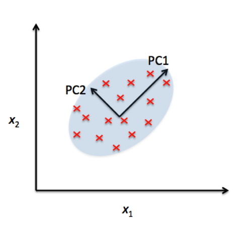
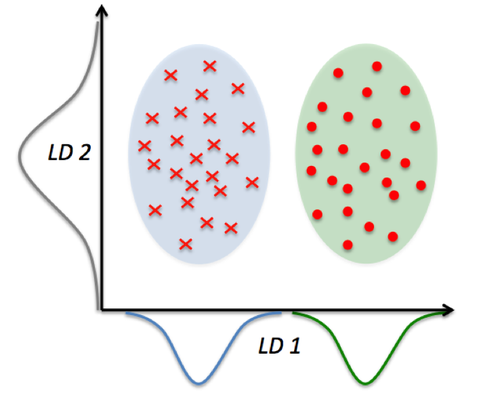
In the comparison above, you can see that PCA reduces on axes (x1,x2) and LDA assumes distributions (LD1, LD2) along the axes. LDA with the LD1 and LD2 components shows better class separability.

You should prefer to use PCA if the data is skewed or irregular (considering the overfitting nature of LDA), and for uniformly distributed data, LDA performs better. However, you can also apply PCA before LDA. Applying PCA can help with regularization and reduce overfitting.

The LDA Algorithm

LDA makes two assumptions for simplicity:

1. The data follows a Gaussian distribution.
2. Each feature/dimension has the same variance Σ.

Following is the LDA Algorithm for the general case (multi-class classification)

Suppose that each of C classes has a mean μ_i, then the scatter between the classes is calculated as:

Here, μ is the average of class means μ_i for i=1…C.

The class separation S along the direction  is given by:

When is an eigenvector of, then S will be equal to the corresponding eigenvalue?

Simply put, if is invertible, the eigenspace corresponding to the C-1 largest eigenvalues will form the reduced space.

Hence, the following steps go into computing an LDA:

1. Compute mean vectors for all C classes in the data (Let dimensions of data=N)
2. Compute the scatter matrices: Σ_w (Covariance within a class) and Σ_b (Covariance between classes)
3. Compute the eigenvalues and eigenvectors for the scatter matrices
4. Select the top k eigenvalues, and build the transformation matrix of size N*k.
5. The resultant transformation matrix can be used for dimensionality reduction and class separation via LDA.

LDA Python Implementation For Classification

In this code, we:

1. Load the Iris dataset in sklearn
2. Normalize the feature set to improve classification accuracy (You can try running the code without the normalization and verify the loss of accuracy)
3. Compute the PCA, followed by LDA and PCA+LDA of the data
4. Visualize the computations using matplotlib
5. Using sklearn RandomForest classifier, evaluate the outputs from Step 2

## dependencies: matplotlib.pyplot, tkinter, and sklearn
# sudo apt-get install python3-tk
# pip install matplotlib sklearn

## load the iris dataset and set up variables
from sklearn import datasets
iris = datasets.load_iris()
iris_features = iris.data
iris_target = iris.target
target_values=sorted(list(set(iris_target)))	# output: [0,1,2]
target_names = iris.target_names	# output: ["setosa","versicolor","virginica"]
del iris

# load up preprocessing
from sklearn.preprocessing import StandardScaler
sc = StandardScaler()
iris_features = sc.fit_transform(iris_features)

## perform PCA of 2 dimensions on the data
from sklearn.decomposition import PCA
pca = PCA(n_components=2)
pca_object = pca.fit(iris_features) # creates a PCA object for (input)
# Returns a new basis*data matrix, X_pca which is reduced to 2 dimensions instead of 4
X_pca = pca_object.transform(iris_features)
del pca_object

## perform LDA of 2 dimensions on the data
from sklearn.discriminant_analysis import LinearDiscriminantAnalysis
lda = LinearDiscriminantAnalysis(n_components=2)
lda_object = lda.fit(iris_features, iris_target) # creates an LDA object for (inputs, targets)
# Returns a new basis*data matrix, like PCA does
X_lda = lda_object.transform(iris_features)
del lda_object

# for comparison against LDA, also perform PCA before doing LDA, then comparison of plots 1 and 3 is possible
lda_object = lda.fit(X_pca, iris_target)
X_pca_lda = lda_object.transform(X_pca)
del lda_object

## Create a plot figure and compare PCA/LDA
import matplotlib.pyplot as plt
fig=plt.figure()
fig.suptitle("Comparison: PCA and LDA") # title of plot

# define a reusable plotting function for plotting data matrices
def subplot_scatter_iris(subplot_location=None, input_matrix=None, title=None, set_legend=True):
	ax=fig.add_subplot(subplot_location)	# add a subplot
    
# create a scatter plot parsing through data points of the matrix, and their corresponding labeled outputs
for i, target in zip(target_values, target_names):
    ax.scatter(input_matrix[iris_target == i, 0], input_matrix[iris_target == i, 1], label=target)
    
if set_legend == True:  # add a legend if set_legend is True
   ax.legend(loc='best',scatterpoints=1)
if title: # add a title if not null
    ax.set_title(title)

# Plot the PCA in location 1, then LDA in 2, then PCA+LDA in 3
subplot_scatter_iris(131, X_pca, "PCA of IRIS dataset", True)
subplot_scatter_iris(132, X_lda, "LDA of IRIS dataset", True)
subplot_scatter_iris(133, X_pca_lda, "LDA applied to PCA of IRIS dataset", True)

## CLASSIFIER - Evaluation of the techniques via confusion matrix
from sklearn.model_selection import train_test_split
from sklearn.ensemble import RandomForestClassifier
from sklearn.metrics import confusion_matrix  
from sklearn.metrics import accuracy_score

classifier = RandomForestClassifier(max_depth=2, random_state=0)

def perform_evaluation(feature_set,target_set):
    def namestr(obj, namespace):
    	    return [name for name in namespace if namespace[name] is obj]
    print("Evaluation for:",namestr(feature_set,globals())[0])
	feat_train, feat_test, target_train, target_test = train_test_split(feature_set, target_set, test_size=0.2, random_state=3)
# pass initial state to generate same indexes

	classifier.fit(feat_train, target_train)
	predicted = classifier.predict(feat_test)
	print("Accuracy: ",accuracy_score(target_test, predicted))
	print(confusion_matrix(target_test, predicted))

perform_evaluation(iris_features, iris_target)
perform_evaluation(X_pca, iris_target)
perform_evaluation(X_lda, iris_target)
perform_evaluation(X_pca_lda, iris_target)
# print evaluation, before drawing the plot
plt.show()

Conclusion

In this article, we focused on understanding LDA and the advantages it offers over PCA. We also looked at an LDA implementation in Python’s Sklearn library on the Iris dataset. In this implementation, we can see comparisons between PCA and LDA, and also that applying PCA before LDA can have its benefits.