

Machine Learning problems involve modeling of Data to uncover the underlying phenomena that is generating the data. This modeling of course is never 100% correct. However, we can say with a certain confidence level that the model is correct. This confidence is often measured in terms of Probability. Therefore, it is important for us to understand various concepts of Probability Theory so as to get a deeper understanding of Machine Learning. In this article we will talk about advanced Machine Learning Probability concepts that are used heavily.
We all know the basics of Probability in that P(E) = n(E) / n(S) where E is the event whose probability is being measured and S is the sample space. The function n(X) represents the size (cardinal number) of the set X.
Random Variables and Machine Learning Probability Distribution
A random variable is a variable whose value is uncertain. It represents outcomes of an experiment. For instance, a random variable X may denote the number of heads obtained when tossing 2 coins. Here, X can take the following values:
0 if we get tail in both tosses.
1 if we get heads in one of the tosses and tail in the other toss.
2 if we get heads in both the tosses.
The probability of getting tail in both tosses is (1/2) x (1/2) = 1/4.
The probability of getting heads in one of the tosses and tail in the other toss is 2 x (1/2) x (1/2) = 1/2.
The probability of getting heads in both tosses is (1/2) x (1/2) = 1/4.
Therefore:
P(X = 0) = 1/4
P(X = 1) = 2/4
P(X = 2) = 1/4
So, we can define a random variable by an associated “Probability Distribution” function F such that FX(x) = P(X = x).
This is the case when the random variable X takes discrete values like 0, 1, 2, etc. However, in certain situations, we have random variables that can take continuous values. In such situations, it makes no sense to define P(X = x). Rather, we talk about Probability of X taking a particular value in an interval around that value. So, FX(x) = P(x <= X <= x + dx). Here, we have chosen the differential interval [x, x + dx] and we are trying to compute the probability that the value of X lies in this interval. This leads us to the concept of Probability density functions. Probability Density
Probability Density of a continuous random variable X is defined as f such that for any measurable set A
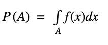
Here, A denotes the set over which we are trying to measure the probability.
As an example, consider the following Probability Density Function:
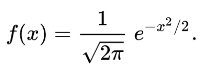
When plotted on the graph, it looks something just like this:
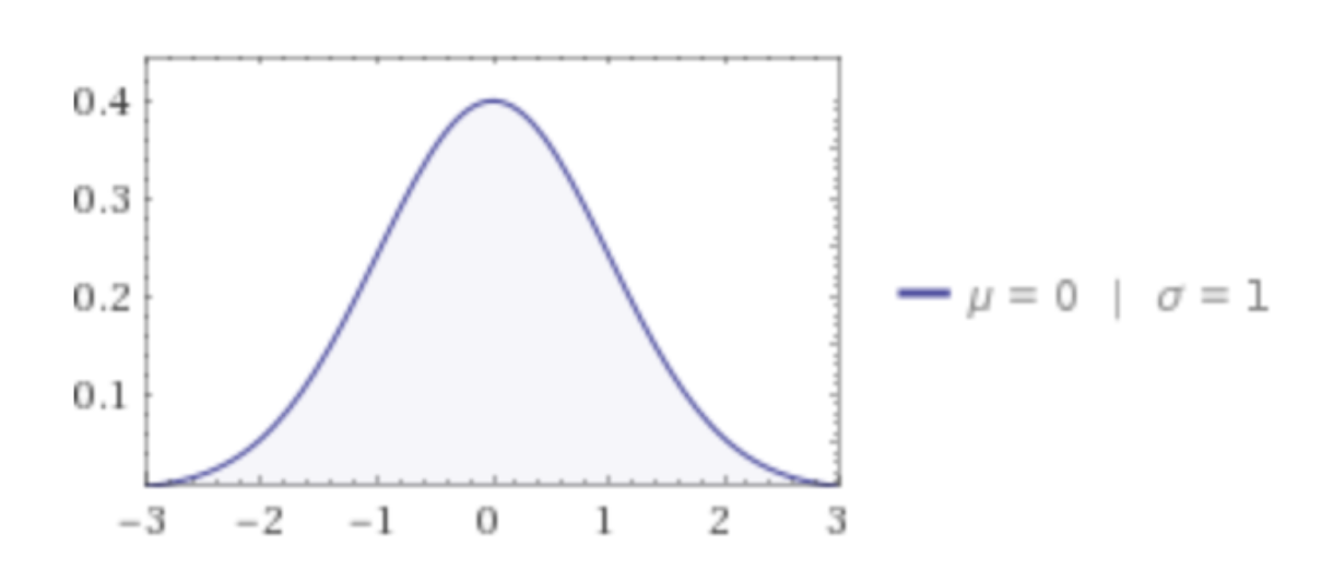
The distribution demonstrated above is termed as the Standard Normal Distribution function. From this distribution, we can derive some important statistics.
Mean: Mean of the random Variable X is defined as:
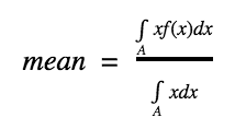
In the numerator, we integrate xf(x) and in the denominator we integrate x which essentially gives us the size of the area over which mean is being calculated. Mean is also called as expectation/expected value and is denoted as E(X). In the above case, the mean turns out to be 0.
Other than mean, we can compute other important statistics also. For instance, one common statistic that is quoted is called as Standard Deviation. Standard Deviation (Sd) is defined as:
Sd(X) = E(X2) – E(X)2
The first term denotes the expected value of the random variable X2 while the second term denotes the square of the expected value of X.
Mean provides an indication of the value where the maximum probability is concentrated. On the other hand, the Standard deviation provides an indication of the “spread” of the density. In the above case, the Standard deviation is 1. As the Standard deviation increases, the graph above spreads more and becomes wider. Mean of the Standard Normal Distribution function indicates the value at which the peak occurs (the top of the bell).
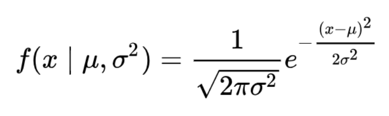
Generalization of the above Standard Normal Distribution is called as the Normal Distribution where mean can be any value ? while standard deviation can be any (positive) value ?.
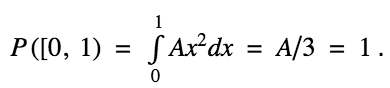
Let us take an example of Probability computation. We are given a continuous random variable in the interval [0, 1]. We are told that the Probability density is given by:
f(x) = Ax2
Here, A is an unknown constant value which we are asked to compute.
We know that Probability of a set A is given as: 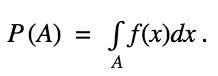
Here, let us choose the set A as the interval [0, 1]. The function f is given as f(x) = Ax2. We know that the total probability of a random variable is nothing but 1. So, we have:
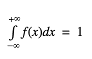
This leads us to an important concept: for any probability density function f(x),
We also have other probability density functions. For instance, for an Exponential Distribution, the Probability Density Function is given as:
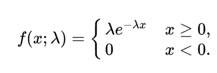
One can easily verify that as per the above equation, the sum total probability turns out to be 1.
Conclusion
Probability as a concept is quite interesting and extremely important. You are advised to familiarize yourself will various types of Probability Density/Distribution functions which widely occur. In particular, the Normal Distribution (also called as Gaussian Distribution) is one of the most well researched Probability Distribution functions. It occurs at multiple places. For instance, daily returns of many stocks follow Gaussian Distribution. Therefore, it is important to understand it thoroughly to develop a sound understanding of various concepts that are covered in Machine Learning domain.

