

In the previous blogs, we covered the basic concept of Generative Adversarial Networks or GANs, along with a code example where we coded up our own GAN, trained it to generate the MNIST dataset from random noise and then evaluated it.
If that blew you away, wait till you’ve followed us to the end of this one.
And if it didn’t, it’s cuz you’ve not given our previous blogs a read (duh!).
So we’ve gone ahead and put the links of the two-part Introduction to GAN blog (Concept and Code) here too, and we highly recommend you go over them. We’d like to again emphasize, once more, that GANs are bleeding edge in Artificial Intelligence for Computer Vision problems. We’ll go as far as to say that almost any interesting paper post-GANs, has a GAN somewhere in it and those statistics will speak more for GANs than we ever can.
More from the Series:

- An Introduction to Generative Adversarial Networks- Part 1
- Introduction to Generative Adversarial Networks with Code- Part 2
- CycleGAN: Taking It Higher- Part 4
- The Grand Finale: Applications of GANs- Part 5
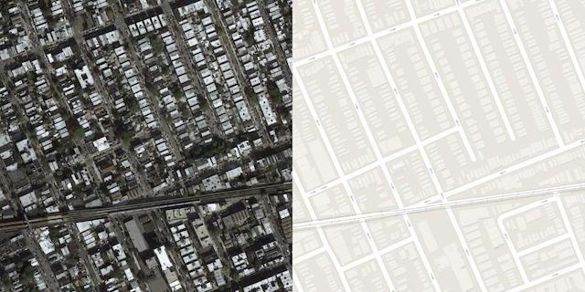
Now, cutting back to this blog and to introduce the agenda for today, we’ll hint the things to come by providing some images below and implore the readers to let loose their imagination to guess what exactly it is that we’ll be accomplishing today:

Alright, readers! Hold all your guesses, our chance now.
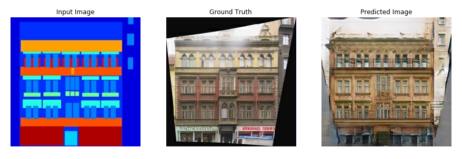
We could make a couple of observations from the preceding image examples:
- We’re generating an image as output as we’d expect with a GAN, but we’re not generating just any image. The image generated at the output takes on certain characteristics, or rather, style of the target image.
- Unlike generating MNIST digits with random N-dimensional noise vectors as input, here the inputs are neither random nor noise and nor N-dimensional. In fact, the input here is also an image.
To sum up the observations in a few sentences, we can say that for the scenario depicted in the images, the output, as well as the input, is controlled and well-defined. This, of course, as previously mentioned, is in direct contrast with what we did with the MNIST dataset where we generated handwritten from N-dimensional random noise vectors, that is, we really had no control over the values in our input.
This is the key difference between the GAN we coded up in our previous blog and the GAN we’ll be coming up here.
Why do we say that the output, as well as the input, is controlled?
This is a simple but important concept.
The reason for the output being controlled is obvious. We say the output is controlled because it is generated based on the training image or the ground truth image (labeled in the preceding image examples). So if you were to change the ground truth to a different image, you’d get a different output, that is, you’d generate a different image. The output is thus guided by the ground truth. That’s basics pretty much. In every type of supervised Neural Networks, the output is guided by the ground truth.
The reason for stating that the input is controlled is because, well, the input in our case is an image and it has a certain sense of structure as opposed to random pixels. That is to say, the input image is not a random gibberish image.
The Goal
The reader would have figured this out following our discussion on the observations and also since it is pretty intuitive from the pictures we’ve provided themselves.
But let’s go ahead and develop the problem statement more precisely.
We’ve said that our input image has a certain sense of structure. Our goal then is to take the structural detail in the input image and essentially translate it to having the same structural detail as the input image but infused with the style of the ground truth image.
We’ll again show one of the examples from preceding images here just so that the reader can read the goal statement (in bold) again and relate it with the images we’ve provided directly so that the goal is absolutely clear before proceeding further.
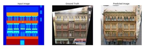
The keyword here being translate. Specifically, image translation.
Let’s talk a bit more about this entire translating business before we proceed further.
What is Image-to-Image Translation?
Image translation is a class of computer vision and graphics problems where the goal is to learn the mapping between an input image and an output image. It can be applied to a wide range of applications, such as style transfer, object transfiguration, season and landscape transfer, artificial coloration, sketches to photo transformation (which is closely related to style transfer), and photo super-resolution.
Read More: Understanding Computer Vision Techniques!
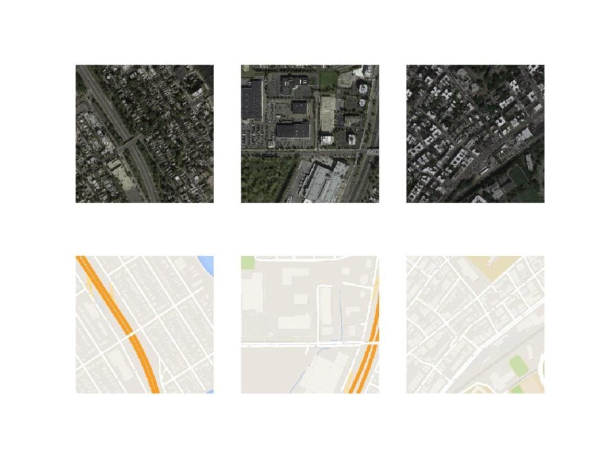
We’ve provided examples for some of the applications below for the clarity of the reader.
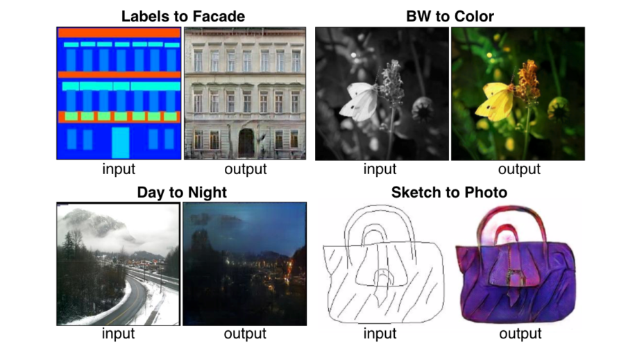
You would have deduced of course, that the images we provided at the beginning of this blog were towards the style transfer domain because that’s where pix2pix GAN comes in.
So, what is the pix2pix GAN?
pix2pix is meant to stand for ‘pixel to pixel’. Essentially, pix2pix is a Generative Adversarial Network, or GAN, designed for general purpose image-to-image translation.
The approach was presented by Phillip Isola, et al. in their 2016 paper titled “Image-to-Image Translation with Conditional Adversarial Networks” and presented at CVPR in 2017.
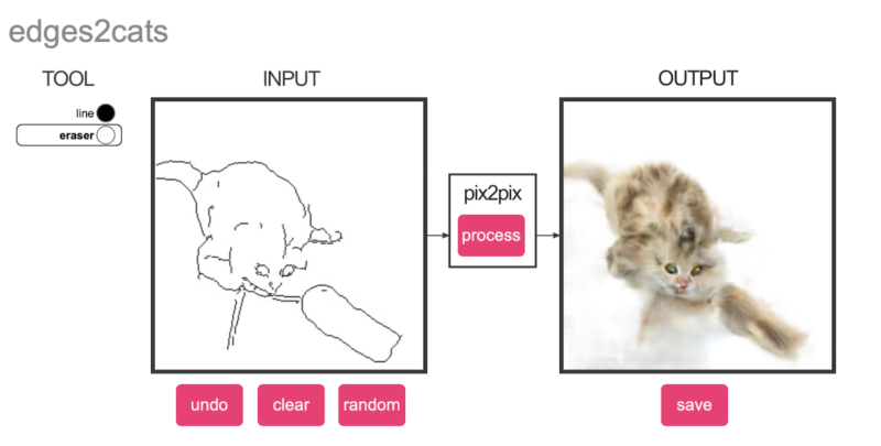
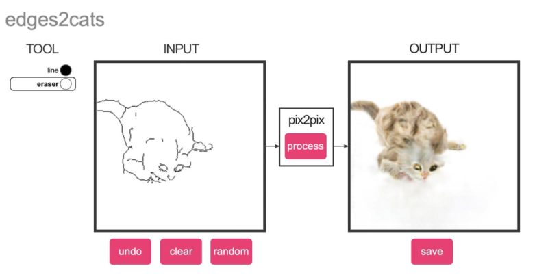
Interestingly, a researcher from the community, Christopher Hesse, has also developed an interactive demo port for everyone to try out and see what the model does for themselves.
We’ll put the link to that right here:
https://affinelayer.com/pixsrv/
We implore the readers to go check this link out where you can see pix2pix in action for the variety of tasks that we described previously. You can give different images as input, modify those images and create your own image and check the output in real-time in a well-designed UI. We have provided a couple of examples that we tried out below:
Now before coming back to the pix2pix GAN, we’d first like to discuss something which is a very important concept and speaks for the uncanny effectiveness that the reader has seen in the example pictures we’ve provided throughout the blog until now. We believe it is important for the reader to thoroughly understand why a simple Convolutional Network cannot give the same uncanny realistic results as a GAN.
It must have been a matter of common observation for our readers, that whenever we’re using a Convolutional Neural Network, we have to designate a certain ‘loss function’ and the Convolutional Neural Networks during training learn to minimize a loss function – an objective that scores the quality of results – and although the learning process is automatic, a lot of manual effort still goes into designing effective losses. In other words, we still have to tell the Network what we wish to minimize.
If we take a naive approach and ask the Network to minimize the Euclidean distance between predicted and ground truth pixels, it will tend to produce blurry results. This is because Euclidean distance is minimized by averaging all plausible outputs, which causes blurring. Coming up with loss functions that force CNN to do what we really want – e.g., output sharp, realistic images – is an open problem and generally requires expert knowledge.
In such cases, it would be highly desirable if we could instead specify only a high-level goal, like “make the output indistinguishable from reality”, and then automatically learn a loss function appropriate for satisfying this goal.
This exactly what GANs in general do and it’s the reason why they’re so effective.
GANs learn a loss that tries to classify if the output image is real or fake, while simultaneously training a generative model to minimize this loss. Blurry images will not be tolerated since they look obviously fake. Because GANs learn a loss that adapts to the data, they can be applied to a multitude of tasks that traditionally would require very different kinds of loss functions.
pix2pix takes this interesting property of GANs and applies it for a general image-to-image translation task developing a new variation of the vanilla GAN that we studied in the previous blogs.
In the pix2pix paper, the authors have explored GANs in a conditional setting. Just as GANs learn a generative model of data, conditional GANs (cGANs) learn a conditional generative model. This makes cGANs suitable for image-to-image translation tasks, where we condition on an input image and generate a corresponding output image.
This is, of course, what we previously observed before where we said that the output images always retained the structure of the input image but infused it with the style of a ground truth image, only now we have a name for such GANs, and they are called cGANs or Conditional GANs.
We’ll now quickly describe the pix2pix GAN architecture before we move on to a real code example as always.
pix2pix GAN Architecture
The pix2pix model is a type of conditional GAN, or cGAN, as we discussed, where the generation of the output image is conditional on input, in this case, a source image. The discriminator is provided both with a source image and the target image and must determine whether the target is a plausible transformation of the source image.
The generator is trained via adversarial loss, which encourages the generator to generate plausible images in the target domain. The generator is also updated via L1 loss measured between the generated image and the expected output image. This additional loss encourages the generator model to create plausible translations of the source image.
It would be perhaps appropriate here to just take a few moments away from the blog and talk about something we believe to be very important when it comes to a field like Artificial Intelligence. You see, Artificial Intelligence is a field that is seeing new frontiers being explored every day. Every day, new research is being carried out that is seeing the development of new architectures, uncovering new optimizations to the existing architectures and new problems are being tackled and solved. The direct consequence of this is that things get obsolete very fast. In such cases, Eduonix recommends each student and each reader to regularly take up interesting research papers so that their knowledge is always true to the state of the art and they invariably become better Artificial Intelligence developers in the long run.
Holding that as preamble, we’d like to use this blog as a starting point to inculcate in the reader the habit of reading research papers.
Even though we’ve designed this blog the way we design all our blogs, which is that they all are always intuitively sufficient to understand the concept as well the implementation, we encourage the reader to start reading research papers herself/himself for the reasons already mentioned. We will provide the link to the paper for this GAN architecture that we would like the reader to go through. We’ve chosen this paper for the reader for the simple reason that this research paper is extremely well written and will not be a heavy read.
https://arxiv.org/pdf/1611.07004.pdf
In the paper, the authors make use of a ‘Maps’ dataset. It is perfectly appropriate for us, then, to work on the same dataset to further strengthen our understanding of the pix2pix GAN and also to see how well we can do with it.
Let the game begin!
As always we’ll begin by a little introduction to the dataset we’ll be using.
The dataset that we’ll be using is comprised of Satellite images of New York and their corresponding Google Maps pages. The image translation problem involves converting satellite photos to Google maps format, or the reverse, Google maps images to Satellite photos.
The dataset is provided on the pix2pix website and can be downloaded as a 255-megabyte zip file.
About the Dataset
The train folder contains 1,097 images, whereas the validation dataset contains 1,099 images.
Images have a digit filename and are in JPEG format. Each image is 1,200 pixels wide and 600 pixels tall and contains both the satellite image on the left and the Google maps image on the right.
Routine Preprocessing
Now as each image is 1,200 pixels wide and 600 pixels tall, it will be difficult to fit a thousand of such images into the RAMs of any modern computer even if it has 16 gigs of RAM memory. So as is the standard procedure, we will resize the images into a manageable dimension of 256×256.
But there’s a small catch here which the sharp reader must have noticed. The dataset images have Satellite Maps and Google Maps in the same image.
It follows then, that we’ll have to, at some point, split the images into the corresponding Satellite and Google Map elements.
Let’s take a quick look at how we can approach this.
#load the required libraries

from os import listdir
from numpy import asarray
from numpy import vstack
from keras.preprocessing.image import img_to_array
from keras.preprocessing.image import load_img
from numpy import savez_compressed

# load all images from the directory into memory with appropriate preprocessing

def load_images(path, size=(256,512)):
	src_list, tar_list = list(), list()
	# enumerate filenames in directory, assuming all are images
	for filename in listdir(path):
		# load and resize the image
		pixels = load_img(path + ‘/’ + filename, target_size=size)
		# convert to numpy array
		pixels = img_to_array(pixels)
		# split into satellite and map
		sat_img, map_img = pixels[:, :256], pixels[:, 256:]
		src_list.append(sat_img)
		tar_list.append(map_img)
	return [asarray(src_list), asarray(tar_list)]
Now to run the above code snippet, all that is required to do is to call the functions we’ve defined as follows:
# dataset path which the users should replace with the paths of their own machine

path = ‘/Users/bhargavdesai/Downloads/maps/train’

# load dataset

[src_images, tar_images] = load_images(path)
print('Loaded: ', src_images.shape, tar_images.shape)

# save as compressed numpy array

filename = 'maps_256.npz'
savez_compressed(filename, src_images, tar_images)
print('Saved dataset: ', filename)
Now just to verify that this approach works, we can, with a few lines of code verify that the images have indeed been formatted just the way that we had envisioned it.
from matplotlib import pyplot

# plot images
n_samples = 3
for i in range(n_samples):
	pyplot.subplot(2, n_samples, 1 + i)
	pyplot.axis('off')
	pyplot.imshow(src_images[i].astype('uint8'))
# plot target image
for i in range(n_samples):
	pyplot.subplot(2, n_samples, 1 + n_samples + i)
	pyplot.axis('off')
	pyplot.imshow(tar_images[i].astype('uint8'))
pyplot.show()
Now that we have prepared the dataset for image translation, we can develop our pix2pix GAN model.
Based on our previous discussion on the architectural details, we know that this model (like any other GAN model) will consist of two components: the discriminator and the generator.
The Discriminator
An interesting approach is undertaken by the authors here in the discriminator model which adds another feature to the pix2pix GAN that allows usage across a variety of image domains.
Readers might reckon that in the previous blog when implementing the discriminator, the discriminator predicted a particular image as ‘fake’ or ‘real’ when we passed the entire image to the deep convolutional network to classify.
Now, unlike the traditional GAN model that uses a deep convolutional neural network to classify images, the pix2pix model uses a PatchGAN. The PatchGAN discriminator is also just a deep convolutional network.
So why is this any different?
Well, this is different because of this deep convolutional neural network designed to classify patches of an input image as real or fake, rather than the entire image.
So basically, this type of discriminator tries to classify if each NxN patch in an image is real or fake. This discriminator is then run convolutionally across the image to return a single feature map of real or fake predictions that can be averaged to give a single score which is the ultimate output of the discriminator.
Now that the concept is clear, let’s take look at the interpretation:
# define the discriminator model

def define_discriminator(image_shape):
	# weight initialization
	init = RandomNormal(stddev=0.02)
	# source image input
	in_src_image = Input(shape=image_shape)
	# target image input
	in_target_image = Input(shape=image_shape)
	# concatenate images channel-wise
	merged = Concatenate()([in_src_image, in_target_image])
	# C64
	d = Conv2D(64, (4,4), strides=(2,2), padding='same', kernel_initializer=init)(merged)
	d = LeakyReLU(alpha=0.2)(d)
	# C128
	d = Conv2D(128, (4,4), strides=(2,2), padding='same', kernel_initializer=init)(d)
	d = BatchNormalization()(d)
	d = LeakyReLU(alpha=0.2)(d)
	# C256
	d = Conv2D(256, (4,4), strides=(2,2), padding='same', kernel_initializer=init)(d)
	d = BatchNormalization()(d)
	d = LeakyReLU(alpha=0.2)(d)
	# C512
	d = Conv2D(512, (4,4), strides=(2,2), padding='same', kernel_initializer=init)(d)
	d = BatchNormalization()(d)
	d = LeakyReLU(alpha=0.2)(d)
	# second last output layer
	d = Conv2D(512, (4,4), padding='same', kernel_initializer=init)(d)
	d = BatchNormalization()(d)
	d = LeakyReLU(alpha=0.2)(d)
	# patch output
	d = Conv2D(1, (4,4), padding='same', kernel_initializer=init)(d)
	patch_out = Activation('sigmoid')(d)
	# define model
	model = Model([in_src_image, in_target_image], patch_out)
	# compile model
	opt = Adam(lr=0.0002, beta_1=0.5)
	model.compile(loss='binary_crossentropy', optimizer=opt, loss_weights=[0.5])
	return model
The define_discriminator() function below implements the PatchGAN discriminator model as per the design of the model in the paper. The model takes two input images that are concatenated together and predicts a patch output of predictions. The model is optimized using binary cross-entropy, and weighting is used so that updates to the model have half (0.5) the usual effect. The authors of Pix2Pix recommend this weighting of model updates to slow down changes to the discriminator, relative to the generator model during training.
Right. So now that’s out of the way, now onto the generator!
The Generator
The generator model is more complex than the discriminator model.
The generator is an encoder-decoder model using a U-Net architecture. We’ll talk a little about the U-Net architecture first as it is one of the most successful models for a variety of tasks but especially in computer vision.
Remember Autoencoders people? To the readers that do, a big thumbs up to you deep learning champions! We’re really proud of you! Keep learning with Eduonix! And to the readers for whom it is the first time here, we would highly recommend you check out our piece on Autoencoders with Keras where we actually walk you through an example so you never forget any concept you learn with us!
Okay. So what is the U-Net model? Let us first look at the schematic and then elaborate on the results.
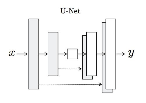
From the schematic, the most basic intuition that can be developed is that the model first downsamples or encodes the input image down to a bottleneck layer, then upsamples or decodes the bottleneck representation to the size of the output image.
But that doesn’t explain the dotted arrows going from the downsampling layers to the upsampling layers. These dotted arrows are called ‘skip connections’ which concatenates the output of the downsampling convolution layers with the feature maps from the upsampling convolution layers at the same level. By the same level, we mean, the same dimension. To be even more concrete, the skip connection from a downsampling layer that has output dimensions, say, 128x128x256 will be concatenated with an upsampling layer that has output dimensions of 128x128x256. Since the network is symmetric, every downsampling layer will have a corresponding upsampling counterpart to facilitate skip connections between.
In our model, the generator, the model takes a source image (e.g. Satellite Map) and generates a target image (e.g. a Google Map).
It does this by first downsampling the input Satellite image down to a bottleneck layer or a very high-level abstract representation, then it upsamples this high-level representation to the size of the output Google Map image which is achieved by the U-Net architecture as we described.
Let’s now look at the implementation details.
# define an encoder block

def define_encoder_block(layer_in, n_filters, batchnorm=True):
	# weight initialization
	init = RandomNormal(stddev=0.02)
	# add downsampling layer
	g = Conv2D(n_filters, (4,4), strides=(2,2), padding='same', kernel_initializer=init)(layer_in)
	# conditionally add batch normalization
	if batchnorm:
		g = BatchNormalization()(g, training=True)
	# leaky relu activation
	g = LeakyReLU(alpha=0.2)(g)
	return g

# define a decoder block

def decoder_block(layer_in, skip_in, n_filters, dropout=True):
	# weight initialization
	init = RandomNormal(stddev=0.02)
	# add upsampling layer
	g = Conv2DTranspose(n_filters, (4,4), strides=(2,2), padding='same', kernel_initializer=init)(layer_in)
	# add batch normalization
	g = BatchNormalization()(g, training=True)
	# conditionally add dropout
	if dropout:
		g = Dropout(0.5)(g, training=True)
	# merge with skip connection
	g = Concatenate()([g, skip_in])
	# relu activation
	g = Activation('relu')(g)
	return g

# define the standalone generator model

def define_generator(image_shape=(256,256,3)):
	# weight initialization
	init = RandomNormal(stddev=0.02)
	# image input
	in_image = Input(shape=image_shape)
	# encoder model
	e1 = define_encoder_block(in_image, 64, batchnorm=False)
	e2 = define_encoder_block(e1, 128)
	e3 = define_encoder_block(e2, 256)
	e4 = define_encoder_block(e3, 512)
	e5 = define_encoder_block(e4, 512)
	e6 = define_encoder_block(e5, 512)
	e7 = define_encoder_block(e6, 512)
	# bottleneck, no batch norm and relu
	b = Conv2D(512, (4,4), strides=(2,2), padding='same', kernel_initializer=init)(e7)
	b = Activation('relu')(b)

# decoder model

	d1 = decoder_block(b, e7, 512)
	d2 = decoder_block(d1, e6, 512)
	d3 = decoder_block(d2, e5, 512)
	d4 = decoder_block(d3, e4, 512, dropout=False)
	d5 = decoder_block(d4, e3, 256, dropout=False)
	d6 = decoder_block(d5, e2, 128, dropout=False)
	d7 = decoder_block(d6, e1, 64, dropout=False)
	# output
	g = Conv2DTranspose(3, (4,4), strides=(2,2), padding='same', kernel_initializer=init)(d7)
	out_image = Activation('tanh')(g)
	# define model
	model = Model(in_image, out_image)
	return model
The encoder and decoder of the generator are comprised of standardized blocks of convolutional, batch normalization, dropout, and activation layers. This standardization means that we can develop helper functions to create each block of layers and call it repeatedly to build-up the encoder and decoder parts of the model.
The define_generator() function below implements the U-Net encoder-decoder generator model. It uses the define_encoder_block() helper function to create blocks of layers for the encoder and the decoder_block() function to create blocks of layers for the decoder. The tanh activation function is used in the output layer, meaning that pixel values in the generated image will be in the range [-1,1].
In this blog, we have assumed an understanding of the layers defined in each blog and the Functional API of Keras. For the more novice readers, we’d recommend brushing up on all the Keras jargon with our Keras series.
Read More:
- Deep Neural Networks with Keras
- Functional API of Keras
- Convolutional Neural Networks with Keras
- Recurrent Neural Networks and LSTMs with Keras
Once the generator model has been defined, we are now ready to define our final composite GAN model which will have both the discriminator as well as the generator working against each other, but also trying to learn from each other as well!
The GAN
This logical or composite model involves stacking the generator on top of the discriminator. A source image is provided as input to the generator and to the discriminator, although the output of the generator is connected to the discriminator as the corresponding “target” image. The discriminator then predicts the likelihood that the generator was a real translation of the source image.
The discriminator is updated in a standalone manner, so the weights are reused in this composite model but are marked as not trainable. The composite model is updated with two targets, one indicating that the generated images were real (cross-entropy loss), forcing large weight updates in the generator toward generating more realistic images, and the executed real translation of the image, which is compared against the output of the generator model (L1 loss).
The define_gan() function below implements this, taking the already-defined generator and discriminator models as arguments and using the Keras Functional API to connect them together into a composite model. Both loss functions are specified for the two outputs of the model and the weights used for each are specified in the loss_weights argument to the compile() function.
# define the combined generator and discriminator model, for updating the generator

def define_gan(g_model, d_model, image_shape):
	# make weights in the discriminator not trainable
	d_model.trainable = False
	# define the source image
	in_src = Input(shape=image_shape)
	# connect the source image to the generator input
	gen_out = g_model(in_src)
	# connect the source input and generator output to the discriminator input
	dis_out = d_model([in_src, gen_out])
	# src image as input, generated image and classification output
	model = Model(in_src, [dis_out, gen_out])
	# compile model
	opt = Adam(lr=0.0002, beta_1=0.5)
	model.compile(loss=['binary_crossentropy', 'mae'], optimizer=opt, loss_weights=[1,100])
	return model
But before proceeding, we’ll define a function to scale the images between [-1,1] because of the presence of the tanh layer in the generator model.
# load image array saved in previous step and prepare training images

def load_real_samples(filename):
	# load compressed arrays
	data = load(filename)
	# unpack arrays
	X1, X2 = data['arr_0'], data['arr_1']
	# scale from [0,255] to [-1,1]
	X1 = (X1 - 127.5) / 127.5
	X2 = (X2 - 127.5) / 127.5
	return [X1, X2]
Training the GAN
Training the discriminator will require batches of real and fake images.
The generate_real_samples() function below will prepare a batch of random pairs of images from the training dataset, and the corresponding discriminator label of class=1 to indicate they are real.
# select a batch of random samples, returns images and target

def generate_real_samples(dataset, n_samples, patch_shape):
	# unpack dataset
	trainA, trainB = dataset
	# choose random instances
	ix = randint(0, trainA.shape[0], n_samples)
	# retrieve selected images
	X1, X2 = trainA[ix], trainB[ix]
	# generate 'real' class labels (1)
	y = ones((n_samples, patch_shape, patch_shape, 1))
	return [X1, X2], y
The generate_fake_samples() function below uses the generator model and a batch of real source images to generate an equivalent batch of target images for the discriminator.
These are returned with the label class-0 to indicate to the discriminator that they are fake.
# generate a batch of images, returns images and targets

def generate_fake_samples(g_model, samples, patch_shape):
	# generate fake instance
	X = g_model.predict(samples)
	# create 'fake' class labels (0)
	y = zeros((len(X), patch_shape, patch_shape, 1))
	return X, y
In our previous blog as well, we’ve made a point regarding the difficulty of training and GAN, particularly its convergence. Typically, GAN models do not converge; instead, an equilibrium is found between the generator and discriminator models. As such, we cannot easily judge when training should stop. Therefore, we can save the model and use it to generate sample image-to-image translations periodically during training, such as every 10 training epochs.
We can then review the generated images at the end of training and use the image quality to choose a final model.
The summarize_performance() function implements this.
# generate samples and save as a plot and save the model

def summarize_performance(step, g_model, dataset, n_samples=3):
	# select a sample of input images
	[X_realA, X_realB], _ = generate_real_samples(dataset, n_samples, 1)
	# generate a batch of fake samples
	X_fakeB, _ = generate_fake_samples(g_model, X_realA, 1)
	# scale all pixels from [-1,1] to [0,1]
	X_realA = (X_realA + 1) / 2.0
	X_realB = (X_realB + 1) / 2.0
	X_fakeB = (X_fakeB + 1) / 2.0
	# plot real source images
	for i in range(n_samples):
		pyplot.subplot(3, n_samples, 1 + i)
		pyplot.axis('off')
		pyplot.imshow(X_realA[i])
	# plot generated target image
	for i in range(n_samples):
		pyplot.subplot(3, n_samples, 1 + n_samples + i)
		pyplot.axis('off')
		pyplot.imshow(X_fakeB[i])
	# plot real target image
	for i in range(n_samples):
		pyplot.subplot(3, n_samples, 1 + n_samples*2 + i)
		pyplot.axis('off')
		pyplot.imshow(X_realB[i])
	# save plot to file
	filename1 = 'plot_%06d.png' % (step+1)
	pyplot.savefig(filename1)
	pyplot.close()
	# save the generator model
	filename2 = 'model_%06d.h5' % (step+1)
	g_model.save(filename2)
	print('>Saved: %s and %s' % (filename1, filename2))
Finally, we can train the generator and discriminator models.
The train() function below implements this, taking the defined generator, discriminator, composite model, and loaded dataset as input.
# train pix2pix model
def train(d_model, g_model, gan_model, dataset, n_epochs=100, n_batch=1):
# determine the output square shape of the discriminator
n_patch = d_model.output_shape[1]
# unpack dataset
trainA, trainB = dataset
# calculate the number of batches per training epoch
bat_per_epo = int(len(trainA) / n_batch)
# calculate the number of training iterations
n_steps = bat_per_epo * n_epochs
# manually enumerate epochs
for i in range(n_steps):
# select a batch of real samples
[X_realA, X_realB], y_real = generate_real_samples(dataset, n_batch, n_patch)
# generate a batch of fake samples
X_fakeB, y_fake = generate_fake_samples(g_model, X_realA, n_patch)
# update discriminator for real samples
d_loss1 = d_model.train_on_batch([X_realA, X_realB], y_real)
# update discriminator for generated samples
d_loss2 = d_model.train_on_batch([X_realA, X_fakeB], y_fake)
# update the generator
g_loss, _, _ = gan_model.train_on_batch(X_realA, [y_real, X_realB])
# summarize performance
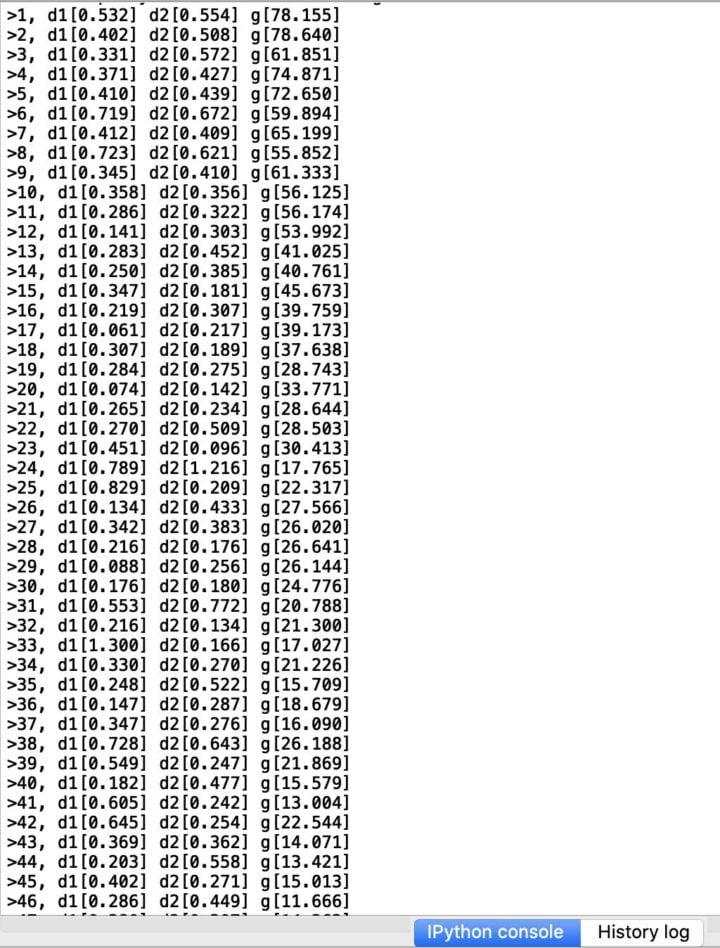
print('>%d, d1[%.3f] d2[%.3f] g[%.3f]' % (i+1, d_loss1, d_loss2, g_loss))
# summarize model performance
if (i+1) % (bat_per_epo * 10) == 0:
summarize_performance(i, g_model, dataset)
Each training step involves first selecting a batch of real examples, then using the generator to generate a batch of matching fake samples using the real source images. The discriminator is then updated with the batch of real images and then fake images.
Next, the generator model is updated providing the real source images as input and providing class labels of 1 (real) and the real target images as the expected outputs of the model required for calculating the loss. The generator has two loss scores as well as the weighted sum score returned from the call to train_on_batch(). We are only interested in the weighted sum score (the first value returned) as it is used to update the model weights.
Finally, the loss for each update is reported to the console each training iteration and model performance is evaluated every 10 training epochs.
Before running the code example, we’d like to request the users to first complete all the necessary imports required which we’ve not included for each individual function since we just wanted to run you through the overall procedure.
# all the necessary imports required

from numpy import load
from numpy import zeros
from numpy import ones
from numpy.random import randint
from keras.optimizers import Adam
from keras.initializers import RandomNormal
from keras.models import Model
from keras.models import Input
from keras.layers import Conv2D
from keras.layers import Conv2DTranspose
from keras.layers import LeakyReLU
from keras.layers import Activation
from keras.layers import Concatenate
from keras.layers import Dropout
from keras.layers import BatchNormalization
from keras.layers import LeakyReLU
from matplotlib import pyplot
Finally, after the necessary imports, let’s run the example by calling each function in the following steps:
# load image data
dataset = load_real_samples('maps_256.npz')
print('Loaded', dataset[0].shape, dataset[1].shape)

# define input shape based on the loaded dataset
image_shape = dataset[0].shape[1:]

# define the models
d_model = define_discriminator(image_shape)
g_model = define_generator(image_shape)

# define the composite model
gan_model = define_gan(g_model, d_model, image_shape)

# train model
train(d_model, g_model, gan_model, dataset)
Results
On running the entire code from start to bottom, we have, at long last, arrived at the training process. A note to our readers, training this GAN takes a very long time on a CPU. We’ve tested the code on an i7 processor clocking at 4.2 GHz with 16 gigs of RAM and it took over 14 hours. While on a GPU hardware, it took less than 2 hours so we’d definitely recommend GPU hardware. In the future, we’ll do a blog covering the training of Deep Neural Networks on GPU hardware since there a lot of cloud services that offer this capability.
Anyway, for now, irrespective of where you runt this code on, you’ll have the following output on your console which is an indicator that the training has begun.
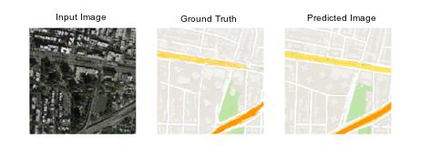
Models are saved every 10 epochs and saved to a file with the training iteration number. Additionally, images are generated every 10 epochs and compared to the expected target images. These plots can be assessed at the end of the run and used to select a final generator model based on generated image quality.
After the first 10 epochs, map images are generated that look plausible, although the lines for streets are not entirely straight and images contain some blurring. Nevertheless, large structures are in the right places with mostly the right colors.
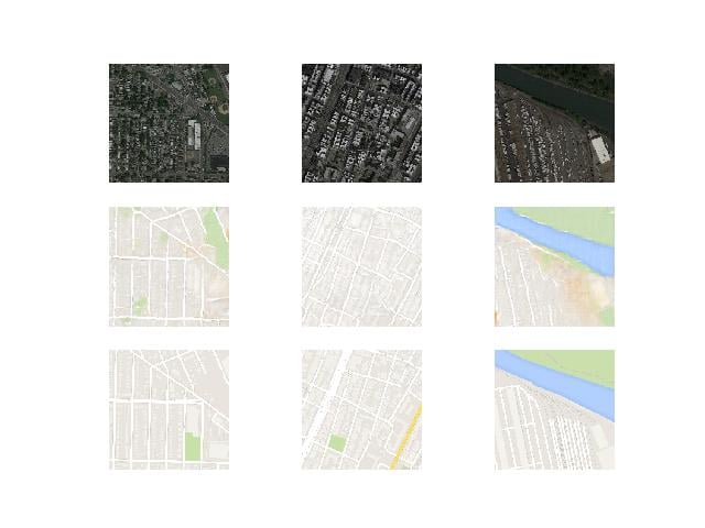
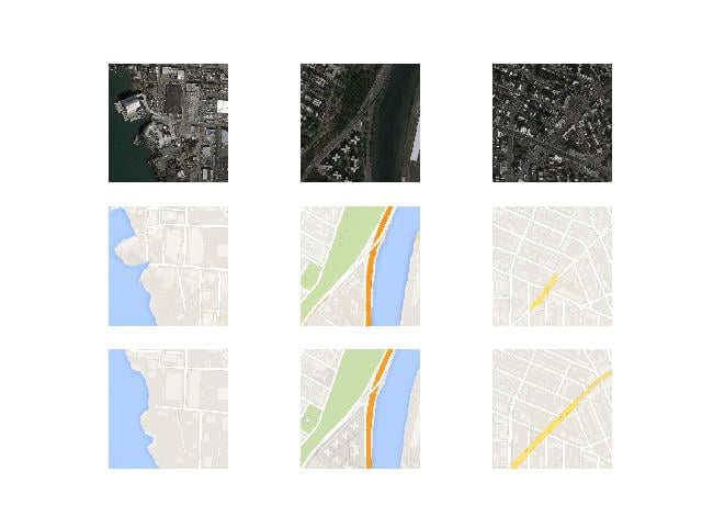
Generated images after about 50 training epochs begin to look very realistic, at least to mean, and quality appears to remain good for the remainder of the training process.
Note the first generated image example below (right column, middle row) that includes more useful detail than the real Google map image.
This effectively concludes this blog on training pix2pix models. In the next blog, we’ll notch things up a bit, taking it even higher by introducing yet another class of problems that can be solved with a completely new architecture of GAN models.
We hope these blogs have got you coding and if not coding, at least got you curious because, at Eduonix, we believe your curiosity is the greatest gift you can give us so we’d very happily take that too.
So looking forward to seeing y’all in the next blog! Don’t miss it for the world! Something BIG is coming, we promise.
More from the Series:
- An Introduction to Generative Adversarial Networks- Part 1
- Introduction to Generative Adversarial Networks with Code- Part 2
- CycleGAN: Taking It Higher- Part 4
- The Grand Finale: Applications of GANs- Part 5
Read More:
- Artificial Intelligence in Space Exploration
- AI Dueling: Witness the New Frontier of Artificial Intelligence
- Artificial Intelligence Vs Business Intelligence
- Role of Artificial Intelligence In Google Android 9.0 Pie
- How Smart Contract can Make our Life Better?
- Why Every Business Should Use Machine Learning?
Looking for Online Learning? Here’s what you can choose from!
- Deep Learning & Neural Networks Using Python & Keras For Dummies
- Learn Machine Learning By Building Projects
- Machine Learning With TensorFlow The Practical Guide
- Deep Learning & Neural Networks Python Keras For Dummies
- Mathematical Foundation For Machine Learning and AI
References:
- Image-to-Image Translation with Conditional Adversarial Networks
- Image-to-Image Translation with Conditional Adversarial Nets
- Unsupervised Image-to-Image Translation Networks
- Implementation of pix2pix in Keras
- PyTorch Implementation
- Convolutional Layers
- Image translation


Really an interesting blog I have gone through. There are excellent details you posted here. Sometime it is not so easy to design and develop a AI and Machine Learning project without custom knowledge; here you need proper development skill and experience. However the details you mention here would be very much helpful for the beginner.