

In this series, we have learned about Dynamic Map creation using ggmap and R, creating dynamic maps using ggplot2, 3D Visualization in R, Data Wrangling and Visualization in R, and Exploratory Data Analysis using the R programming language.
This will be the last article of this series on R programming language wherein we will know about Clustering using FactoExtraPackage.
Clustering is a type of unsupervised machine learning pattern. An unsupervised learning method is considered as a method in which helps us to draw references from data-sets which consists of input data without labeled responses. Generally, it is considered as a process to find meaningful structure, explanatory underlying processes and the required generative features with respect to inherent features.
Clustering involves the task of dividing the population or data points of the mentioned data-set into a number of groups such that data points in the same groups are considered more similar to other data points in the same group and in the same fashion dissimilar to the data points in other groups. Clustering includes a collection of objects on the basis of similarity and dissimilarity between them.
The best demonstration for clustering is the data points in the graph below clustered together can be classified into one single group. We can distinguish the clusters as mentioned in the figure mentioned below:
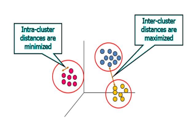

Intracluster distance is the sum of distances between objects in the same cluster. This distance should always be minimized. Intercluster distance is the distance between objects in a different cluster. This distance should always be maximized.
Importance of Clustering
Clustering is very important as it determines the intrinsic grouping among the unlabeled data which is present. Hence, it is considered as a supervised machine learning pattern. There are no specific criteria for good clustering. It depends on the specific user who has the criteria through which requirements are satisfied. The best demonstration can be taken as finding representatives for similar data groups for finding “natural clusters” and describe their unknown properties in finding different groups and finding unusual data objects (outlier detection).
Types of Clustering Algorithms
It is now equally important to understand clustering methods include methods that are used to deal with a large amount of data. There are two types of clustering which are explained below:
1. Hierarchical clustering: The clusters formed in this method forms a tree-type structure based on the hierarchy.
These find successive clusters using previously established clusters.
Agglomerative algorithms begin with each element as a separate cluster and merge them into successively larger clusters. It is also called a “bottom-up” approach. Divisive is also called the “top-down” algorithm to begin with the whole set and proceed to divide it into successively smaller clusters.
2. Partitional clustering: Partitional algorithms determine all clusters at once and randomly. It includes K-means and derivatives -k means algorithm can handle a large number of data points.
Let us follow the below-mentioned steps to implement the clustering method with FactoExtra package in R.
Step 1: Install the necessary packages which is required for creating clusters in R.
> install.packages("factoExtra")
> install.packages("cluster")
Step 2: Include the required libraries in the R workspace to implement the clustering procedure.
> library(factoextra)
> library(cluster)
> data(USArrests)
> USArrests <- na.omit(USArrests)
> # View the first 6 rows of the data
> head(USArrests, n = 6)
           Murder Assault UrbanPop Rape
Alabama      13.2     236       58 21.2
Alaska       10.0     263       48 44.5
Arizona       8.1     294       80 31.0
Arkansas      8.8     190       50 19.5
California    9.0     276       91 40.6
Colorado      7.9     204       78 38.7
Step 3: Create a module of descriptive statistics which includes minimum, median, mean, standard deviation, and maximum values.
> desc_stats <- data.frame(
+     Min = apply(USArrests, 2, min), # minimum
+     Med = apply(USArrests, 2, median), # median
+     Mean = apply(USArrests, 2, mean), # mean
+     SD = apply(USArrests, 2, sd), # Standard deviation
+     Max = apply(USArrests, 2, max) # Maximum
+ )
> desc_stats <- round(desc_stats, 1)
> desc_stats
          Min   Med  Mean   SD   Max
Murder    0.8   7.2   7.8  4.4  17.4
Assault  45.0 159.0 170.8 83.3 337.0
UrbanPop 32.0  66.0  65.5 14.5  91.0
Rape      7.3  20.1  21.2  9.4  46.0
Step 4: Scaling is an important feature for clustering as it focuses on creating the value range with a specific limit and allows us to maintain the intercluster and intracluster distance properly as defined in the condition mentioned above.
The formula for scaling the variables mentioned in the data frame is to subtract variable from mean and divide by their standard deviation t
scaled _parameter = x-mean/standard deviation
> df<-scale(USArrests)
> df
                    Murder     Assault    UrbanPop         Rape
Alabama         1.24256408  0.78283935 -0.52090661 -0.003416473
Alaska          0.50786248  1.10682252 -1.21176419  2.484202941
Arizona         0.07163341  1.47880321  0.99898006  1.042878388
Arkansas        0.23234938  0.23086801 -1.07359268 -0.184916602
California      0.27826823  1.26281442  1.75892340  2.067820292
Colorado        0.02571456  0.39885929  0.86080854  1.864967207
Connecticut    -1.03041900 -0.72908214  0.79172279 -1.081740768
Delaware       -0.43347395  0.80683810  0.44629400 -0.579946294
Florida         1.74767144  1.97077766  0.99898006  1.138966691
Georgia         2.20685994  0.48285493 -0.38273510  0.487701523
Hawaii         -0.57123050 -1.49704226  1.20623733 -0.110181255
Idaho          -1.19113497 -0.60908837 -0.79724965 -0.750769945
Illinois        0.59970018  0.93883125  1.20623733  0.295524916
Indiana        -0.13500142 -0.69308401 -0.03730631 -0.024769429
Iowa           -1.28297267 -1.37704849 -0.58999237 -1.060387812
Kansas         -0.41051452 -0.66908525  0.03177945 -0.345063775
Kentucky        0.43898421 -0.74108152 -0.93542116 -0.526563903
Louisiana       1.74767144  0.93883125  0.03177945  0.103348309
Maine          -1.30593210 -1.05306531 -1.00450692 -1.434064548
Maryland        0.80633501  1.55079947  0.10086521  0.701231086
Massachusetts  -0.77786532 -0.26110644  1.34440885 -0.526563903
Michigan        0.99001041  1.01082751  0.58446551  1.480613993
Minnesota      -1.16817555 -1.18505846  0.03177945 -0.676034598
Mississippi     1.90838741  1.05882502 -1.48810723 -0.441152078
Missouri        0.27826823  0.08687549  0.30812248  0.743936999
Montana        -0.41051452 -0.74108152 -0.86633540 -0.515887425
Nebraska       -0.80082475 -0.82507715 -0.24456358 -0.505210947
Nevada          1.01296983  0.97482938  1.06806582  2.644350114
New Hampshire  -1.30593210 -1.36504911 -0.65907813 -1.252564419
New Jersey     -0.08908257 -0.14111267  1.62075188 -0.259651949
New Mexico      0.82929443  1.37080881  0.30812248  1.160319648
New York        0.76041616  0.99882813  1.41349461  0.519730957
North Carolina  1.19664523  1.99477641 -1.41902147 -0.547916860
North Dakota   -1.60440462 -1.50904164 -1.48810723 -1.487446939
Ohio           -0.11204199 -0.60908837  0.65355127  0.017936483
Oklahoma       -0.27275797 -0.23710769  0.16995096 -0.131534211
Oregon         -0.66306820 -0.14111267  0.10086521  0.861378259
Pennsylvania   -0.34163624 -0.77707965  0.44629400 -0.676034598
Rhode Island   -1.00745957  0.03887798  1.48258036 -1.380682157
South Carolina  1.51807718  1.29881255 -1.21176419  0.135377743
South Dakota   -0.91562187 -1.01706718 -1.41902147 -0.900240639
Tennessee       1.24256408  0.20686926 -0.45182086  0.605142783
Texas           1.12776696  0.36286116  0.99898006  0.455672088
Utah           -1.05337842 -0.60908837  0.99898006  0.178083656
Vermont        -1.28297267 -1.47304350 -2.31713632 -1.071064290
Virginia        0.16347111 -0.17711080 -0.17547783 -0.056798864
Washington     -0.86970302 -0.30910395  0.51537975  0.530407436
West Virginia  -0.47939280 -1.07706407 -1.83353601 -1.273917376
Wisconsin      -1.19113497 -1.41304662  0.03177945 -1.113770203
Wyoming        -0.22683912 -0.11711392 -0.38273510 -0.601299251
Step 5: Once the values are scaled for the mentioned data-frame, we can implement the k-means algorithm. The steps to be implemented for k-means is mentioned below:
The way the k-means algorithm works is as follows:
- Include the number of clusters with specific number K.
- Initialize centroids by the random shuffle of the dataset and then randomly selecting the required K data points from the centroids without replacement.
- Complete the iteration until there is no change to the centroids.
> set.seed(123)
> km.res <- kmeans(df, 4, nstart = 25)
> head(km.res$cluster, 20)
    Alabama      Alaska     Arizona    Arkansas  California    Colorado Connecticut
          1           4           4           1           4           4           3
   Delaware     Florida     Georgia      Hawaii       Idaho    Illinois     Indiana
          3           4           1           3           2           4           3
       Iowa      Kansas    Kentucky   Louisiana       Maine    Maryland
          2           3           2           1           2           4
Note: The kmeans() function is in-built within the “FactoExtra” package of R.
Step 6: Visualize the cluster as it is required to see the data format which is created as mentioned below:
> fviz_cluster(km.res, USArrests)
> res.km <- eclust(df, "kmeans")
Clustering k = 1,2,..., K.max (= 10): .. done
Bootstrapping, b = 1,2,..., B (= 100)  [one "." per sample]:
.................................................. 50
.................................................. 100
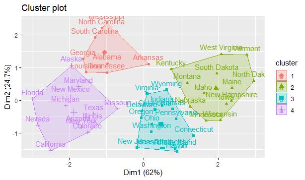
The 4 clusters are created as per the geographical area which includes various aspects and features of the crime rates which are generated.
So, this was it from the R Programming Series!!
Other articles from this series:
- Dynamic Map creation using ggmap and R
- Creating dynamic maps using ggplot2
- 3D Visualization in R
- Data Wrangling and Visualization in R
- Exploratory Data Analysis using R


