

Linear Regression Model is a technique used to model the relationship between a continuous response variable and continuous or categorical predictor(s). The response variable can also be referred to as the dependent variable while the predictor variable can also be referred to as the independent variable. When there is only one independent variable, the resulting model is referred to as simple linear regression. When there are two or more independent variables, the model is referred to as multiple linear regression
A simple linear regression model has the form shown below:
y = β0 + β1×1 + ε
Where y is the dependent variable, x1 is the independent variable, β0 and β1 are coefficients and ε are residuals or errors
A multiple linear regression model has the form shown below
y = β0 + β1×1 + β2 x2 + β1×1 + ε
Where y is the dependent variable, x1 , x2 , x3 are independent variables β0 , β1 , β2 , β3 are coefficients and ε are residuals or residuals
In practice, there will always be more than one independent variable therefore, this tutorial will focus on multiple linear regression.
For a regression model to be reliably used in prediction or making inference about parameters there are assumptions that need to be satisfied. The assumptions are discussed below.
The residuals are required to be normally distributed
The residuals are required to be homoscedastic i.e variance is constant over time, predictions and any independent variable
The errors are not auto-correlated
The relationship between dependent and independent variables is linear and additive
When any of the assumptions is violated there are several techniques that can cure the problem. When the linearity or additivity assumption is violated prediction on data not used in model building will be very inaccurate. Non-linearity is examined using a plot of residuals or observed values against predicted observations. The linearity assumption is valid when observations are symmetrically distributed along a line with a constant variance. Non-linearity can be remedied by applying a log transformation on variables, adding a non-linear term or adding an independent variable that helps in explaining non-linear relationship.
Auto-correlated errors are a sign of a model that is not correctly specified and needs improvement. Autocorrelation is examined using a time series plot of residuals. Another approach to detect auto-correlation is using Durbin-Watson statistic. Ideal values of the statistic are close to 2.
When constant variance (homoscedasticity) assumption is violated, confidence intervals of predictions are unstable. Constant variance is examined using a plot of residuals against predicted values. An increase in residuals across predicted values is evidence of non-constant variance that needs to be corrected. A commonly used approach to correct increasing variance is applying a log transformation on dependent variable.
When the normality of residuals is violated, hypothesis tests on model coefficients and confidence intervals of forecasts are unreliable. Normality violation is very serious when making inference about coefficients, but is not of much concern in prediction. Normality is visually examined using a density plot or a normal quantile plot.
Besides checking assumptions it is also very important to investigate the presence of outliers or extreme observations.
To demonstrate linear regression in using R, we will use the diabetes data available on kaggle. The data is available on this link https://www.kaggle.com/uciml/pima-indians-diabetes-database/data. We will understand the relationship between blood glucose and other recorded patient characteristics.
Use the code below to load the data and view it
diabetes <- read.csv("C:/Users/INVESTS/Downloads/pima-indians-diabetes-database/diabetes.csv")
View(diabetes)
We will use box plots to visualize the distribution of each variable in the data. A sample code of glucose variable is shown below. Use it to visualize the other variables. The boxplot helps us identify observations that need further investigation.
ggplot(diabetes, aes(x=1, y=Glucose)) + geom_boxplot() + xlim(c(0.5,1.5)) +
stat_summary(fun.y=mean, colour="darkred", geom="point",
             shape=18, size=3) + geom_jitter()
To fit a regression model, we use the code shown below
diabetes.model = lm(Glucose ~ Pregnancies + BloodPressure + SkinThickness + Insulin + BMI + DiabetesPedigreeFunction + Age, data = diabetes)
summary(diabetes.model)
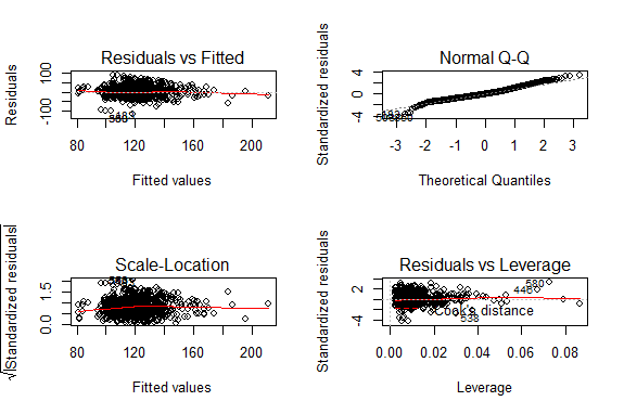
Before making inference using the fitted model, we need to check model assumptions. The diagnostic plots are produced using the code below
par(mfrow=c(2,2)) # visualize the four plots at once
plot(fit)
The residuals vs fitted plot is used to examine the assumption of constant variance. The residuals are not symmetric about the red line and they appear to decrease as fitted values increase. The constant variance assumption was violated and corrective measures are needed. The plot did not reveal a non-linear relationship so the linearity assumption was not violated. The normal Q-Q plot is used to assess normality. In this case there appeared to be no deviation from normality assumption. The scale-location plot is also suitable for assessing constant variance assumption. The residuals vs leverage plot is used to examine presence of extreme observations. Any values outside Cook’s distance need further investigation. Our model did not have extreme observations.
The resulting model is shown below
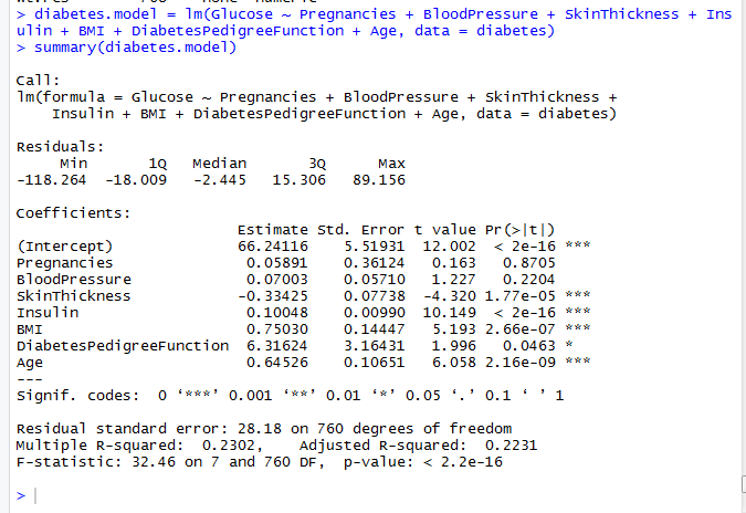
Interpretation of the regression model begins by looking at the F-statistic which tests if there are independent variables that are significant. In this model, the p value is less than 0.05 so we conclude there are some significant independent variables. When there are no significant independent variables the model is not useful for making inference about the coefficients. Multiple R-squared shows the percentage of variation a model is able to explain. Our model was able to explain 23.02% of variation in the data.
To infer if there are independent variables that significantly influence dependent variable we look at t tests of individual coefficients. Skin thickness, insulin, diabetes pedigree function and age had p values less than 0.05. Therefore they were significant predictors of blood glucose. When a coefficient is positive the effect of the independent variable is to increase the dependent variable. When a coefficient is negative the effect of the independent variable is to decrease the dependent variable. In our model, skin thickness decreased blood glucose while the other variables increased blood glucose.
In this tutorial, the simple and multiple linear regression models were introduced. The assumptions that a linear regression model needs to satisfy were discussed. The consequences of violating the assumptions as well as the techniques were discussed. The diabetes dataset available on kaggle was used to demonstrate model fitting, checking assumptions and interpretation.

