

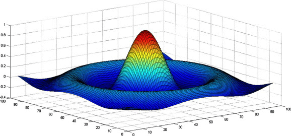
 Algorithms for neural networks depend on the application and the type of the dataset. Hence, the complexity of the use case becomes the deciding factor for the neural network structure. This article will discuss the Mexican Hat neural network with a competitive type of learning technique and a different structure than the traditional ones.
Supervised learning has always been a better approach concerning training a model. Sometimes, the dataset has input values, so there has to be a technique to detect the patterns and relationships between the input data points as the target values are not available for such type of dataset. Hence, unsupervised learning becomes an effective technique to such kinds of datasets and use cases. Generally, classification and clustering problems are handled using unsupervised learning. Mexican Hat neural network is also a part of the unsupervised learning technique.
Competitive learning is an essential concept in terms of unsupervised learning, including classification or clustering problems. The competitive learning principle focuses on asserting that a particular part/layer of the neural network has an excitatory or maximum response on processing the input data. Hence, this part/layer of the neural network is selected for further computations, and the winner layer of neurons is selected at the end of this competition. Mexican Hat uses a similar algorithm but instead of a particular layer of neurons, a bubble around that layer is considered to be the winner.
The architecture of Mexican Hat Neural Network
The neurons are attached with the excitatory positive weights to the neurons closer to the reference neuron. Similarly, the neurons are also connected with negative inhibitory weights with neurons at a farther distance. In some architectures, some neurons are further away still which are not connected in terms of weights. “All of these connections are within a particular layer of a neural net.” The neural network acquires external input data apart from these connections. This data is multiplied with the corresponding weights depending on the proximity to obtain the value. This will be more clear after discussing the algorithm.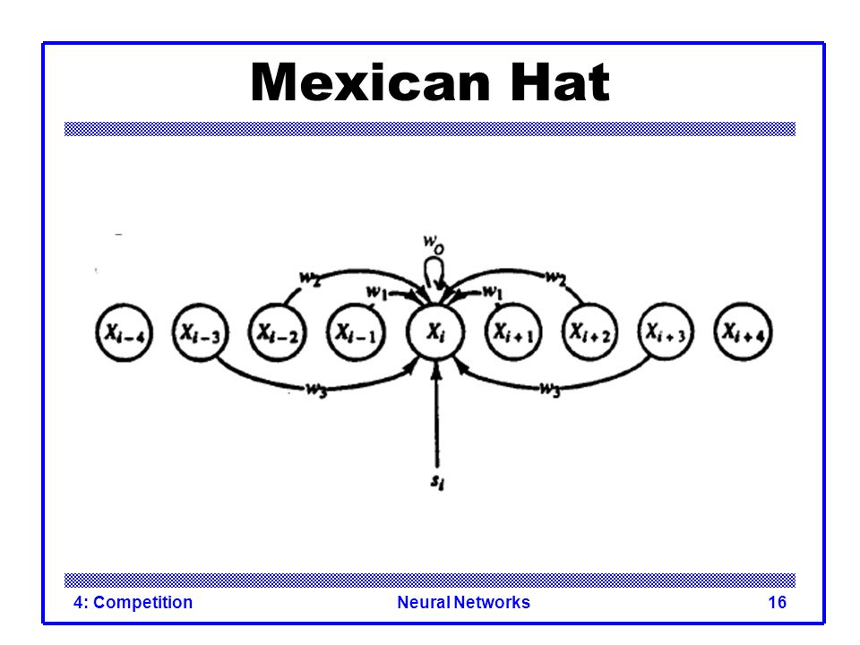
Algorithm for Mexican Hat Neural Network
Let ‘R1’ be the radius of reinforcement, the area closer to the reference neuron. ‘R2’ be the radius of connection further away from the reference neuron where R1 < R2.
Wk represents the weight of the neighbors that varies according to the proximity of the neuron.
Variation conditions are:
- Wk is positive if 0 < k ≤ R1
- Wk is negative if R1 < k ≤ R2
- Wk is zero if k > R2
‘X’ and ‘X_old’ be the vector of activations of the current and previous epoch. Finally, ‘t_max’ be the total number of “iterations of contrast enhancement.”
- Step 1: Depending on the use case, initialize the values of R1, R2, and t_max.
Now, set the initial weights of the neural network
Wk = C1 for k = 0, 1, 2, R1, where C1 > 0.
Wk = C2 for k = R1+1,R1+2,….,R2 where C2 < 0
- Step 2: For the first iteration, set the external signal vector X=S
Fix the activations in the X_old array for i = 1, 2, n, to be used in the next epoch.
- Step 3: Find the overall input for i =1, 2, n.
(net)i = Xi = C1∑ (x_old)i+k – C2 ∑ (x_old)i+k – C2 ∑(x_old) i+k
- Step 4: Apply the activation function and save current activations in X_old for using it in the next iteration.
- Step 5: Increase the counter variable t, as t = t +1.
- Step 6: Test for stopping condition:
If t < t_max, then continue (Go to step 3), else stop.
Brute Force Approach for the Algorithm
The brute force approach for implementing the algorithm is directly applying the mathematical algorithm. This technique does not take care of the time and space complexities, as the ultimate goal is to get the correct results. The algorithm starts by defining all the variables at the start of the program.
As we would be using the NumPy array so it is necessary to import the “numpy” package. According to the algorithm R1, R2, C1, C2, and tmax values could be assumed randomly according to your wish. Make sure that C1>0 and C2<0 as it is the main concept of the algorithm as discussed in the previous section. We have defined a nine-element numpy array for the external input signal with symmetrical but random values. It is also important to append some extra zeroes according to our R1 and R2 values. This allows easier implementation of the algorithms when we are using the loop for calculations.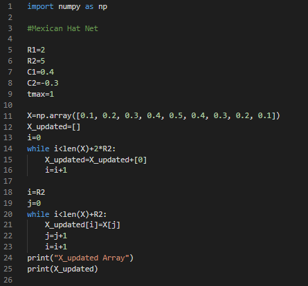
Initialize the variables for tracking the iterations for the while loop. Also, create an array with all zero values for storing the calculated values after each iteration. The first while loop goes through each element of the external input signal. Further, we have three while loops inside the first while loop. These while loops are according to the conditions of the nearby and far weights. Hence, the element values are multiplied with C1 and C2 depending on the position of the element and are added to the main sum. This sum is the actual updated value for an element’s instance of the external input signal. Finally, after passing each element through the calculations we will get an updated vector as our result.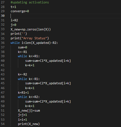
Optimized Approach for the Algorithm
For optmizing the algorithm the time complexity can be reduced from the brute force algorithm. Instead of using the while loop for adding extra zeroes, we can directly append certain number of zeroes to the array by using the np.zeroes() method. As we know that C1 would be used for closer elements and C2 would be used for far elements. So, a weight array can be created according to the number of elements and the definition of activation.
One of the reasons for the time complexity is the usage of nested loops for implementing the algorithms. In brute force algorithm we used nested while loops for calculating the addition of the multiplied weight values with the input element values. But for optimized algorithm we will use a single loop followed by dot product calculation to avoid the usage of nested while loops. This reduces the time complexity significantly. This technique is similar to the sliding window algorithm. Also, this could be reduce the space complexity as we are using less variables in this case. This would be more clear by reviewing the below code. 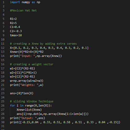
Code for Brute Force Algorithm
import numpy as np


#Mexican Hat Net


R1=2

R2=5

C1=0.4

C2=-0.3

tmax=1


X=np.array([0.1, 0.2, 0.3, 0.4, 0.5, 0.4, 0.3, 0.2, 0.1])

X_updated=[]

i=0

while i<len(X)+2*R2:

    X_updated=X_updated+[0]

    i=i+1

i=R2

j=0

while i<len(X)+R2:

    X_updated[i]=X[j]

    j=j+1

    i=i+1

print("X_updated Array")

print(X_updated)


#updating activations

t=1

converge=0


i=R2

j=0

X_new=np.zeros(len(X))

print('')

print("Array Status")

while i<len(X_updated)-R2:

    sum=0

    k=-R1

    while k<=R1:

        sum=sum+C1*X_updated[i+k]

        k=k+1


    k=-R2

    while k<-R1:

        sum=sum+C2*X_updated[i+k]

        k=k+1

    k=R1+1

    while k<=R2:

        sum=sum+C2*X_updated[i+k]

        k=k+1

    X_new[j]=sum

    j=j+1

    i=i+1

    print(X_new)
Output
Code for Optimized Algorithm
import numpy as np


#Mexican Hat Net


R1=2

R2=5

C1=0.4

C2=-0.3

tmax=10


# creating a Xnew by adding extra zeroes

X=[0.1, 0.2, 0.3, 0.4, 0.5, 0.4, 0.3, 0.2, 0.1]

Xnew=[0]*R2+X+[0]*R2

print("Input: ",np.array(Xnew))


# creating a weight vector

w1=[C2]*(R2-R1)

w2=[C1]*(2*R1+1)

w3=[C2]*(R2-R1)

w=np.array(w1+w2+w3)

print("Weights: ",w)


ans=[0]*len(X)


# sliding Window Technique

for i in range(0,len(X)):

    Xnew=list(Xnew)

    ans[i]=np.dot(w,np.array(Xnew[i:i+len(w)]))

print("Output: ",ans)

print([-0.15,0.04 , 0.33, 0.51, 0.58 , 0.51 , 0.33 , 0.04 ,-0.15])
Output 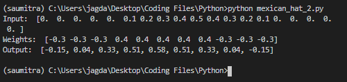
Also Read: How AI Algorithms Have Changed the Car Marketplace Online?

