

Although there is no universally agreed data science process, there are five key steps in a data science workflow. These are illustrated in the flow diagram below
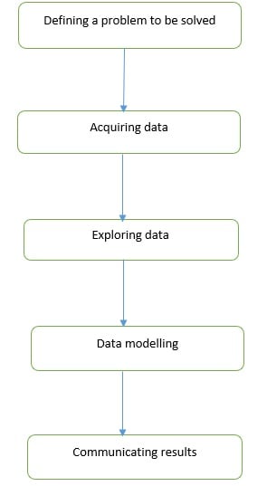
Defining a problem to be solved: While defining a problem, you focus on challenges faced by your organization. In this step you avoid any data modelling considerations.
Acquiring Data: You focus on importing data into your Python environment.
Exploring Data: You focus on understanding data, identifying and addressing data quality problems.
Data modelling: You use an iterative approach of comparing different models to find a model that best explains the relationship between your variables.
Communicating results: You explain your results to decision makers to facilitate decision making or to a software development team so they can develop a data science product.
Introduction to Python
Python is a general-purpose computer programming language that offers rich functionality for data science. You can use either Python 2 or Python 3 for data science functioning. The selection of the version can be done based on the availability of packages and/or any requirements to support legacy code.
There are some minor syntax differences between the two Python versions. Earlier, Python 2 had a distinct advantage i.e. all the packages were available for usage. But now, all the packages are ported to Python 3. Also, let me inform that the Python 2.7 support will expire by the end of 2019. So it is advisable to go for Python 3.
How to set up a data science environment?
Due to many dependencies that need to be satisfied when installing individual packages, it is advisable to use a Python distribution instead of building a data science environment from scratch. Available Python distributions are ‘Anaconda’, ‘Enthought Canopy Express’, ‘PYTHONXY’ and ‘WINPYTHON’. The latter two distributions mentioned are Windows only solutions.
Anaconda and Enthought are offered as a free or paid product. For this tutorial we will use the following Anaconda distribution (https://www.anaconda.com/download/). Download your preferred version and install.
A complete list of available packages are: https://docs.anaconda.com/anaconda/packages/pkg-docs/. Please check the version you are downloading has all the packages you need.
Introduction to Conda
‘Conda’ is a package management tool available in Anaconda that simplifies searching, installing and managing packages together with their dependencies. Conda is also an environment manager that you can use to create separate environments running different Python versions. Another feature of Conda is it can be used together with continuous integration systems such as Travis VI and AppVeyor to support automated code testing. Conda is bundled with all versions of Anaconda, Miniconda and Anaconda repository.
How to install a package?
Click on the title of the package to the installusing the structure conda install PACKAGENAME.
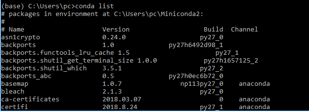
To list available packages in your environment, use the command conda list.
If the package of your choice is unavailable, you can easily install it using conda. To demonstrate this we will install the packages scipy, scikit, matplotlib, tensorflow and keras. The commands to complete this are shown below.
Before attempting to install a package, you can check its availability using the command conda search PACKAGENAME. For example, to search for scipy use the command conda search scipy. The command will provide a list of all available packages.
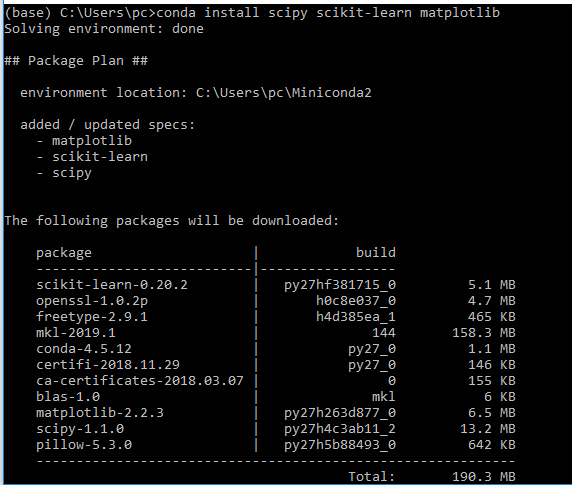
To install all packages at once use the command below
conda install scipy scikit-learn matplotlib
To specify a package version use the command below
conda install scipy=0.19.0 scikit-learn=0.19.0 matplotlib=2.0.2
Introduction to Pip
When your desired package is unavailable in conda or in Anaconda.org you can use pip to install it. Pip is bundled with Anaconda and miniconda, so a separate install is not necessary. Installing packages via pip is done in a similar way as installing via conda. Just pass the package name using the construct pip install PACKAGENAME.
Introduction to Jupyter notebooks
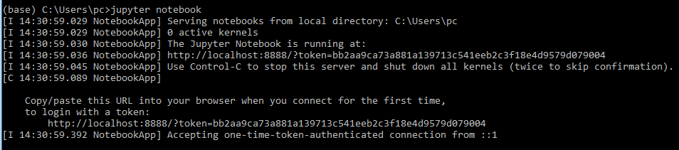
Although there are many IDEs that support Python, a better way of working with data science code is Jupyter notebooks. A Jupyter notebook is an open source web application that supports creation and sharing of code. Jupyter notebook allows you to create code and documentation, run code and see results. Because of the completeness of the environment you are able to complete a workflow that involves data acquisition, exploration, cleaning and modelling. Jupyter is bundled with Anaconda so there is no extra installation step. To start a Jupyter notebook issue the command jupyter notebook at Anaconda prompt. A web page will be opened in your default browser providing you access to Jupyter notebooks.
Data Science workflow
The previous sections introduced data science workflows and demonstrated how to set up a data science environment. After completing the sections it is expected you have a working environment. The following sections will introduce data acquisition, exploration, cleaning and modelling.
After clearly defining ‘a problem to be solved’, the next step is getting the data into your environment. The core package for data acquisition in a Python data science workflow is ‘Pandas’. Pandas provides two data structures that you use to organize your data. These are dataframe and Series objects. A dataframe object organizes data using rows and columns similar to the way a spreadsheet organizes data. A small example is shown below
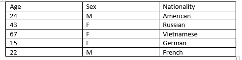
A series object organizes data as an indexed array. An example of a series object storing temperature observed at different times of the day is shown below
![]()
The most common data sources in data science are flat files (spreadsheets, text files and JSON) and relational databases. Flat files are easily imported by specifying the file name and options such as delimiter and column name. The commonly used functions for reading text files are read_csv and read_table. To practice reading in data, download global tuberculosis burden data reported by WHO: https://www.who.int/tb/country/data/download/en/
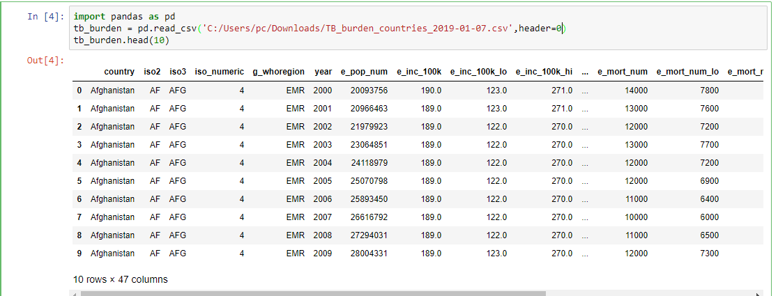
Create a Jupyter notebook and use the commands below to read in data and display the first 10 rows of data.
import pandas as pd
tb_burden = pd.read_csv(‘C:/Users/pc/Downloads/TB_burden_countries_2019-01-07.csv’,header=0)
tb_burden.head(10)
When data is stored in a relational database, Pandas enables you to read a table or results of a query into a dataframe. To read a table you pass the table name, connection object and schema to read_sql_table function. To store query results in a dataframe you pass the query and connection object to read_sql_query function.
*As this is an introduction level tutorial all data input and output functions cannot be discussed. A complete reference is available here https://pandas.pydata.org/pandas-docs/stable/api.html#sql
Data Exploration in detail
After reading in data the next step in a workflow is data exploration. The objective here is to understand your data and identify anomalies. Some of the issues you might come across are missing values, range of observations and relationships among variables. In Pandas missing values can either be standard or not standard. Standard missing values are represented as NA therefore Pandas automatically detects them as missing values. To check for standard missing values you use the function isnull. To get the count of missing values in each column of TB data you use the command print tb_burden.isnull().sum()
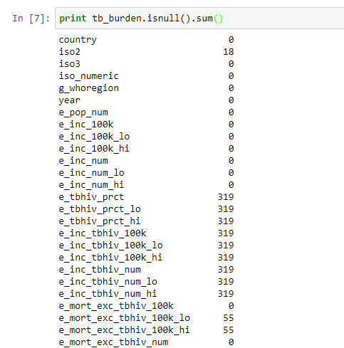
Missing values report shows there are columns with very many missing values. The cause of these missing values needs to be investigated and corrected before further analysis.
Non-standard missing values are more difficult to detect and there is no standard approach to detect them. Thus, Investigative skills are required to identify them.
A quick statistical summary of your data will give you an idea of data distribution and if there are out of range observations. To get a statistical summary of TB data the command tb_burden.describe()
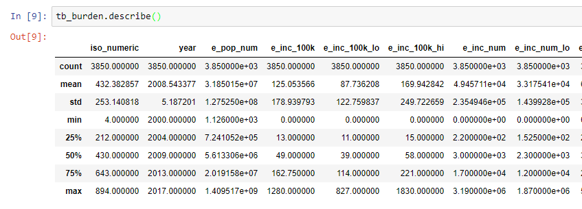
For example, The obtained data was from 2008 to 2017 and hence, the years are within an acceptable range. If the data was from 2020, then that would be a suspicious value.
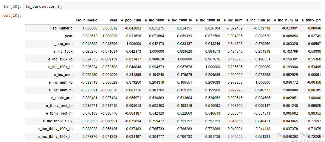
To get the correlation of numeric variables in TB data the command tb_burden.corr() is used. A correlation characterizes the relationship between two numerical variables. It can be used simply to understand the relationship between two variables or as a guide to select variables that are included in a linear regression model.
Another approach to data exploration is visualizing data using graphs. In Python data, visualization can be done using ‘Matplotlib’, ‘Bokeh’, ‘Seaborn’ and ‘ggplot’ among others. To visualize a single numerical variable a histogram or boxplot is used. To visualize a categorical variable a bar chart or pie chart is used. To visualize one or more numerical variables over time a line plot is used. To visualize the relationship between two numerical variables a scatterplot is used.
In this tutorial we will show a few examples of visualizing data using matplotlib. To create a histogram of mortality associated with TB the code below can be used
from matplotlib import pyplot as plt
plt.hist(tb_burden[‘e_mort_100k’])
plt.xlabel(‘Estimated mortality of TB cases (all forms) per 100 000 population’)
plt.ylabel(‘Frequency’)
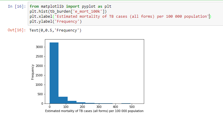
From the histogram above, it can be observed that most countries had mortality below 100 cases per 100000 people with very few countries having a mortality of more than 300 cases per 100000 people.
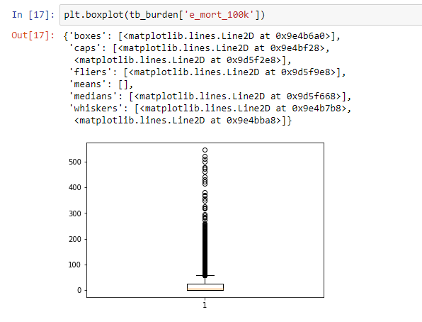
We can visualize the same information using a boxplot. A box plot as shown below considers most of the values above 100 to be outliers, confirming the earlier observation most countries had mortality cases lower than 100. This is an example of skewed data where there are a few countries with very high mortality cases.
A complete reference of available visualizations in Matplotlib is available here http://www.scipy-lectures.org/intro/matplotlib/matplotlib.html.
Building a Model
After getting a good understanding of your data and resolving data-quality problems, the next step is building a model. The scikit-learn package provides an environment for model building and evaluation. Both supervised or unsupervised models can be developed.
Supervised model: a model is given labelled examples from which it learns and predicts on unseen data. Available models in scikit are linear regression, logistic regression, random forests, support vector machines and nearest neighbors, among others. A complete reference of supervised models is available here https://scikit-learn.org/stable/supervised_learning.html.
Unsupervised model: The objective is to automatically discover the underlying structure of data. Some of the available models are clustering, principal components analysis and factor analysis among others. A complete reference is available here https://scikit-learn.org/stable/supervised_learning.html.
Bottom Line
In this tutorial data science workflows were introduced. Use of Python for data science was introduced and setting up a Python environment was demonstrated. Importing data from flat files and relational databases was discussed. Statistical and graphical techniques for data exploration were briefly discussed. Finally available models were discussed.

