

Analyzing an algorithm can help us discover different characteristics, which can help us evaluate its capability for various applications or can be used to compare it with other algorithms for the same application to choose one that’s efficient.
Performance analysis
The computational complexity addresses the resources needed to run the algorithm;
Two types of complexities are essential for analyzing the complexities of algorithms given below.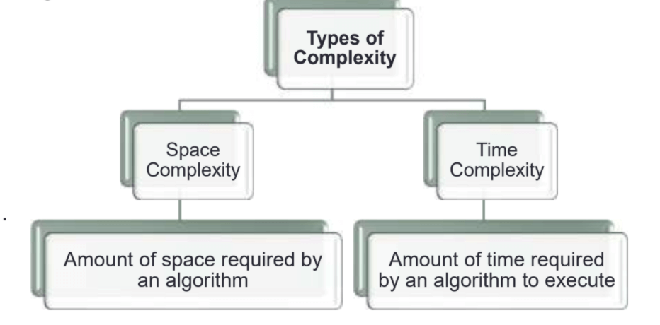
Space Complexity-
An algorithm that uses less memory is better as it can:
- Run-on cheaper hardware (less RAM).
- Have a more significant number of different algorithms running on the same hardware
The amount of memory required to run an algorithm is essential when processing large datasets (such as Big Data). While designing embedded systems, the cost and size of hardware components should be minimum.
Time Complexity-
The faster an algorithm can solve a problem, the better. The time cost has an impact on the financial cost of running an algorithm as:
- Computers consume electricity to run
- A quicker program could solve more of the same problem or run more programs in the same period.
For example, imagine how a ‘slower’ algorithm can affect the financial cost of running a commercial application hosted on a cloud-based server where processing time is supposed to be credited.
Time and Space Complexity of Sorting Algorithms-
INSERTION SORT
Algorithm -Sort the array in ascending order:
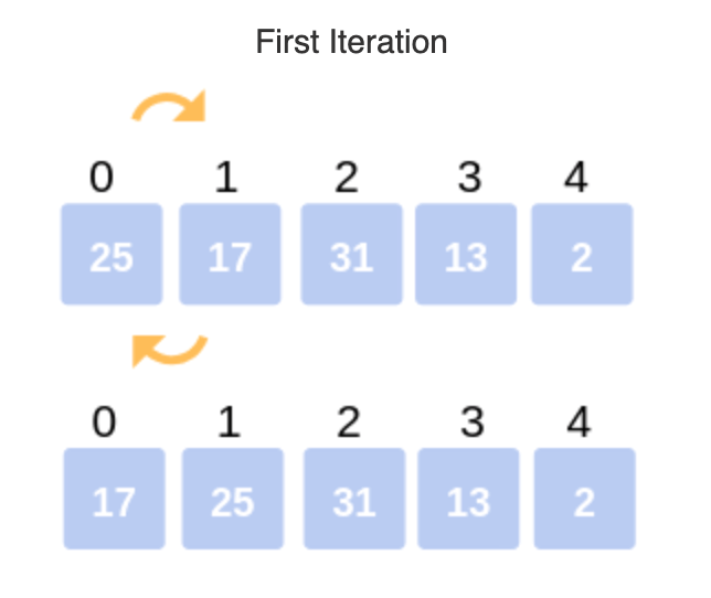
1: Iterate from arr[1] to arr[n] over the array.
2: Compare the current element (key) to its predecessor.
3: If the critical element is smaller than its predecessor, compare it to the parts before. Move the more significant pieces one position up to make space for the swapped element.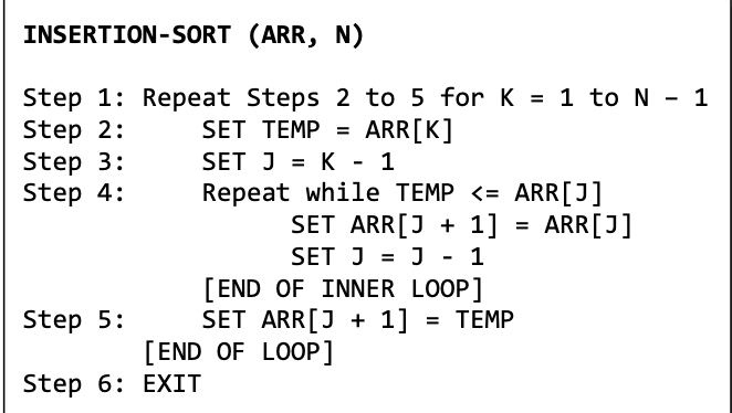
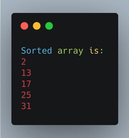
IMPLEMENTATION

Time Complexity
In insertion sort, The sorted array is the best case. In this case, the algorithm’s running time has a linear running time O(n). Hence, every iteration of the nested loop will shift the elements of the sorted set of the array before inserting the next element. The worst case, in insertion sort, has a quadratic running time O(n2).
Space Complexity
Since this algorithm modifies the array in place without using additional memory, it has a space complexity of O(1).
MERGE SORT
Merge sorting uses a divide, conquer and combine approach.
Divide the n-element array into two sub-arrays of n/2 elements. Conquer means sorting the two sub-arrays recursively using merge sort. Combine means merging the two sorted subarrays of size n/2 to produce the sorted array of n elements.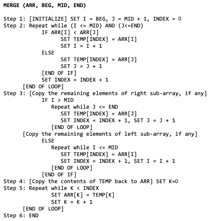
ALGORITHM- 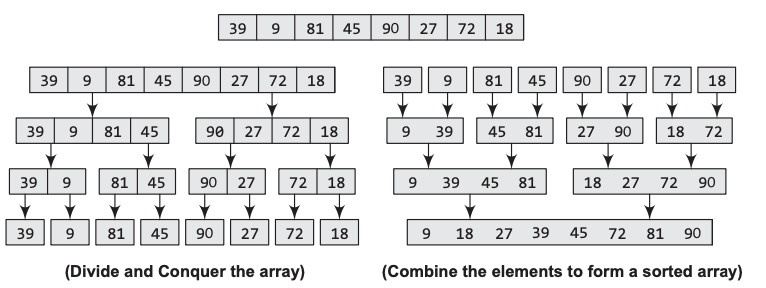
IMPLEMENTATION-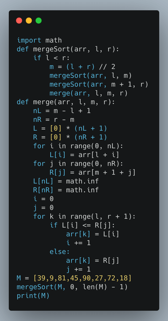
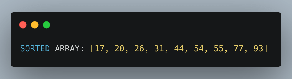
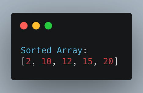
OUTPUT-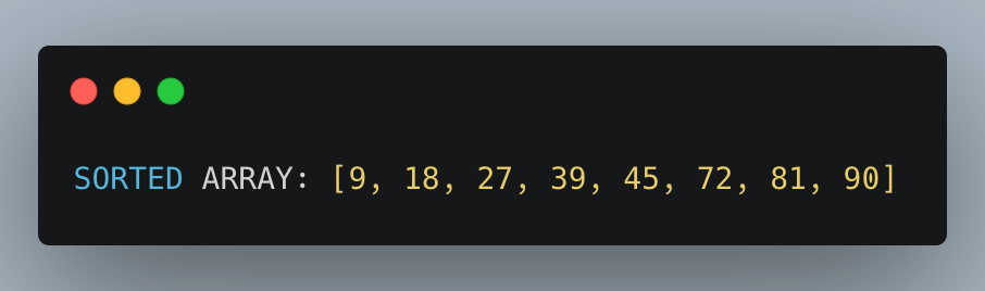
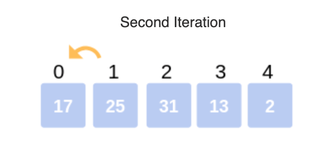
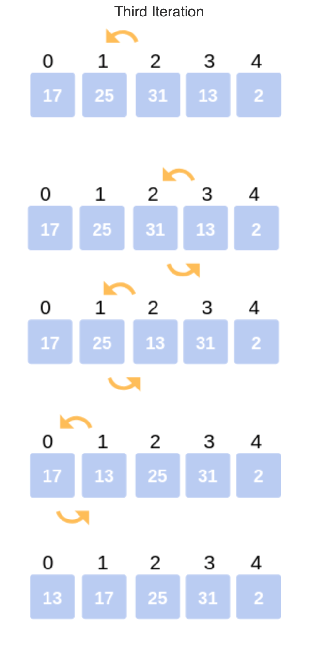
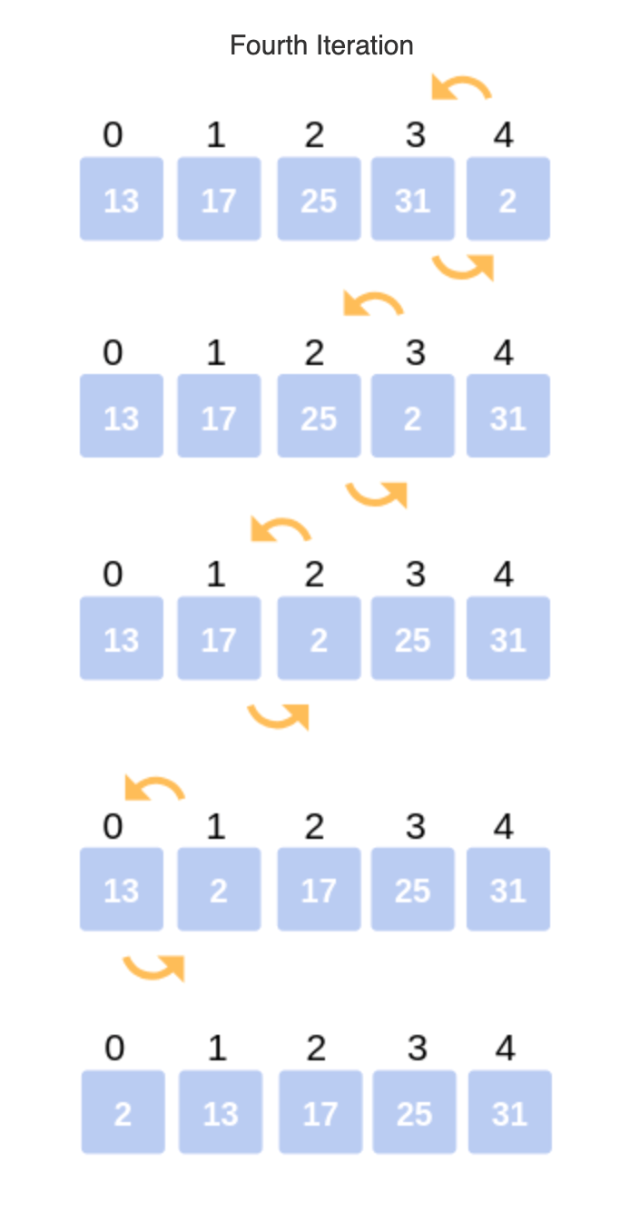
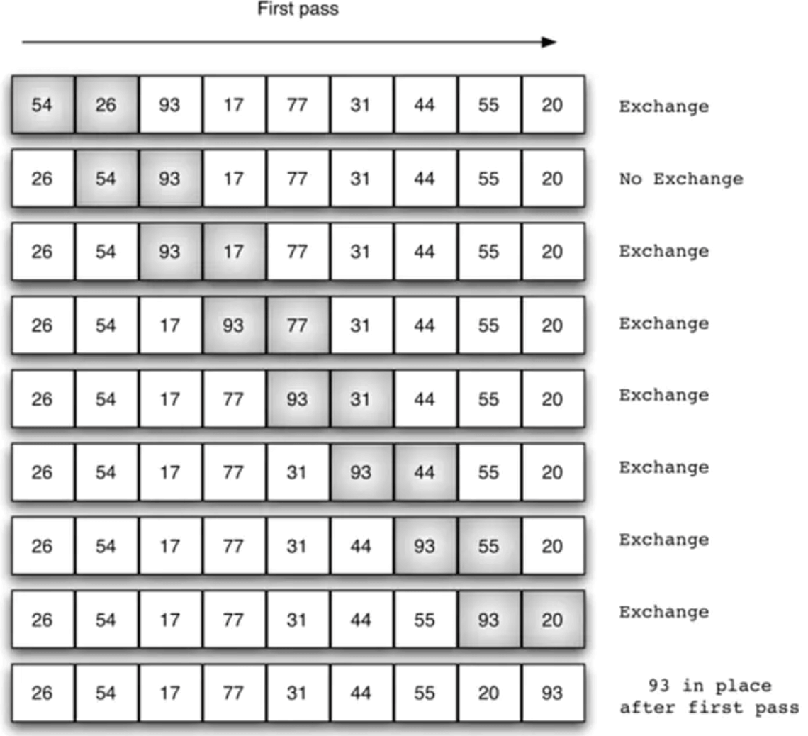
Bubble Sort
In this method, Elements are swapped if the element at the lower index is more significant than the higher index. This process will continue till the list of unsorted elements exhausts.
ALGORITHM-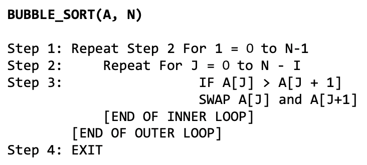
 IMPLEMENTATION-
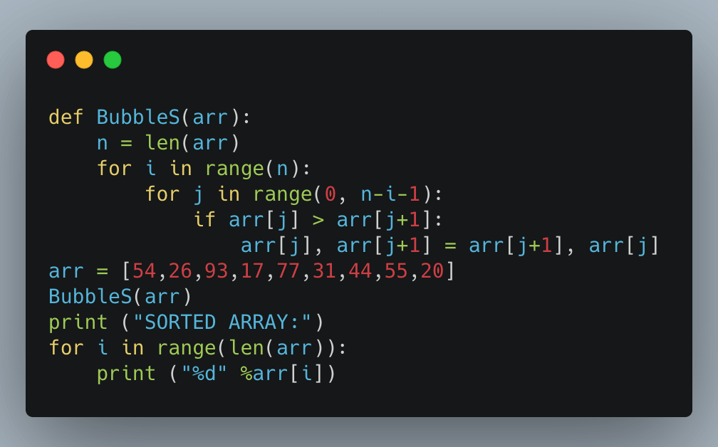
 Time Complexity-
To calculate the total number of comparisons. It can be given as:
f(n) = (n – 1) + (n – 2) + (n – 3) + ….. + 3 + 2 + 1 f(n) = n (n – 1)/2
f(n) = n2/2 + O(n) = O(n2)
Space Complexity-
Bubble sort has a constant space complexity of O(1).
Selection Sort
Selection sort is an algorithm that has a quadratic running time complexity of O(n2)
ALGORITHM-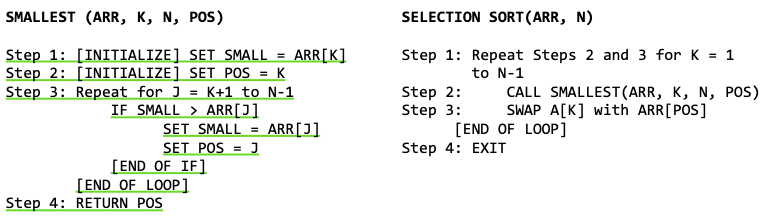
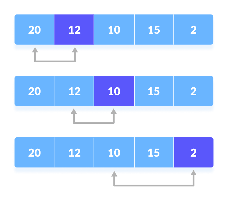
IMPLEMENTATION-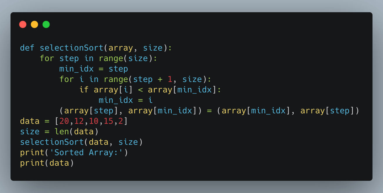
Time complexity-
Selecting the element with the smallest value. N –1 comparisons are required. Then the element is swapped with the smallest value with the first position. In Pass 2, selecting the second smallest value requires scanning the remaining n – 1 element and so on. Therefore,
(n – 1) + (n – 2) + … + 2 + 1
= n(n – 1) / 2 = O(n2) comparisons
Space Complexity
Selection sort modifies the original list. Therefore, it has a constant space complexity of O(1).
COMPARISON OF SORTING ALGORITHMS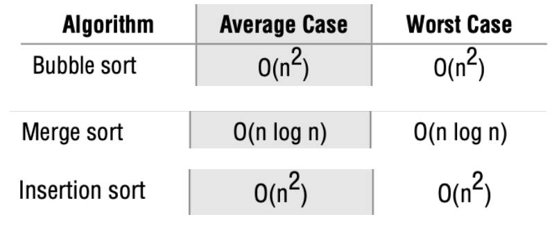 Order of growth is the time of execution depending on the length of the input. In the above example, we can see that the time of performance linearly depends on the size of the array. It helps us to compute the running time efficiently. We use different notations to describe the limiting behavior of a function.
Different notations are used for limiting the behavior of a function.l
Big O
It describes the upper bound of the complexity of an algorithm. It helps to calculate the worst-case of an algorithm. It is necessary to compare outcomes of worst case and best case complexity. While determining the space complexity of an algorithm, two tasks are implemented-
Task 1: We need to implement the program for a particular algorithm.
Task 2: We need to know the size of the input.
Omega Ω
It describes the lower bound of the complexity. It helps to calculate the best time an algorithm can take to complete its execution, i.e., it also helps to measure the best case time complexity of an algorithm. It determines what the fastest time that an algorithm can run is.
Theta Θ
It describes the exact bound of the complexity. It carries the middle characteristics of both Big O and Omega notations as it represents an algorithm’s lower and upper bound.
It helps to know the value of the worst-case and the best-case is the same.
It is a method to know both the upper and lower bound of an algorithm running time.
Whenever an algorithm does not perform worst or best in real-world problems, algorithms mainly fluctuate between the worst-case and best-case, which gives us the average case of the algorithm.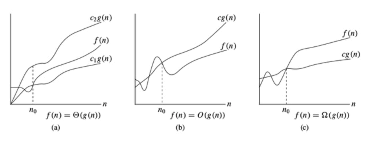 CONCLUSION
As we have seen, time and space complexity depends on hardware, processors, etc. However, we consider the execution time of an algorithm rather than these factors while analyzing the algorithm.
We can conclude that recognizing the best possible algorithms to solve a particular problem should be the one that requires less memory space and takes less time to complete its execution to solve problems. There can be multiple approaches to resolve an issue. If it requires less memory space, then the CPU execution time will be decreased.
Hence, if an algorithm contains loops, then the efficiency of that algorithm may vary depending upon the number of loops running in the algorithm.
So, if space is a constraint, then one might choose a program that takes less space at the cost of more CPU time. On the contrary, if time is an important constraint, Selecting a program that takes minimum time to execute can be more efficient.
Also Read: Learn How to Work with R Data Structures