

SSUCv3H4sIAAAAAAACA01Ry2rDQAz8FbFn0we9+dZDKBQKoe0t9KDsKrbIemW0aych+N+rTdLQ2+g5o9HZbTGzd+3ZcYxTLoqFJbn2uXEUuIgyRtc+LY3LBcuUKVuvRR4LdVa9xH9LNuead637Jt8nidKdnA1OW0utIvmikthntzT3xp7gVUu+t31w9hQjJpLJGn8ahx0lf6qsRqsUCS8iNlbaHwrpcFM0cyC5QpwCV+hm8Rit/lIV23Uy1GynOPbslWfSGgfK3oAzIbxjbxcDp2IquFITcJaBirIHL8MomatFcODSg+9R0ZsKkB2obKVc8yNGKoUgKB44dRbbRgMZzCoKYPN2iCaDdBzJfKxEs1kkCv8/8QArewNuI8Fq/QWYAnxSCkbICd7Xb7ATHczKxpVjNdQ1N2evu/JjIC911UxWkr19dlmWX59XdNz3AQAA
Convolutional neural networks (CNNs) are a form of deep neural network that is widely used in various applications and domains and is particularly useful for evaluating visual imagery in deep learning. When compared to ANNs, CNNs are more effective and require less computation. CNN captures the spatial features from an image. The arrangement of pixels and their relationship in an image is referred to as spatial features. They help us in accurately identifying an object as well as its position and relationship to other objects in a picture.
CNN consists of an input layer, hidden layers and an output layer. The building blocks of CNN are filters (a.k.a kernels) that detect particular features in an image. In other words, filters are nothing but feature detectors. A convolution operation is performed on the image and the filter. The resulting matrix or grid is a feature map that indicates the position of that particular feature in the image. Multiple filters are convoluted with the image to produce numerous feature maps, which can then be convoluted further with more filters to detect every image. The ‘relu’ activation function is applied to the feature maps to introduce non-linearity to the model. The beauty of CNN is that the model involves the filters automatically, so we don’t have to code it from scratch. The only things that need to be defined are the number of filters and their sizes.
To minimize computational load, the size of the feature maps is also reduced by pooling operations. Pooling decreases the size of feature maps while not affecting their ability to detect the features in the image. Together, pooling and convolution provide position invariant feature detection, making the model tolerant towards minor distortions and variations.
An ultimately linked dense neural network for classification is used in the next segment. The feature maps or images are flattened into a one-dimensional array. This flattened output is fed into a feed-forward neural network, which is then trained using backpropagation.
This article will briefly demonstrate training a CNN to classify CIFAR images using the Tensorflow library in python programming.
Dataset for Training and Testing the CNN Model
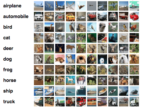
We will use the CIFAR10 dataset, which contains 60,000 colour images (32×32) in 10 classes, each class consisting of 6,000 images. The dataset is split into 50,000 training images and 10,000 test images. The classes are mutually exclusive i.e. there is no overlap between any two classes.
Designing the Convolution Neural Network Model
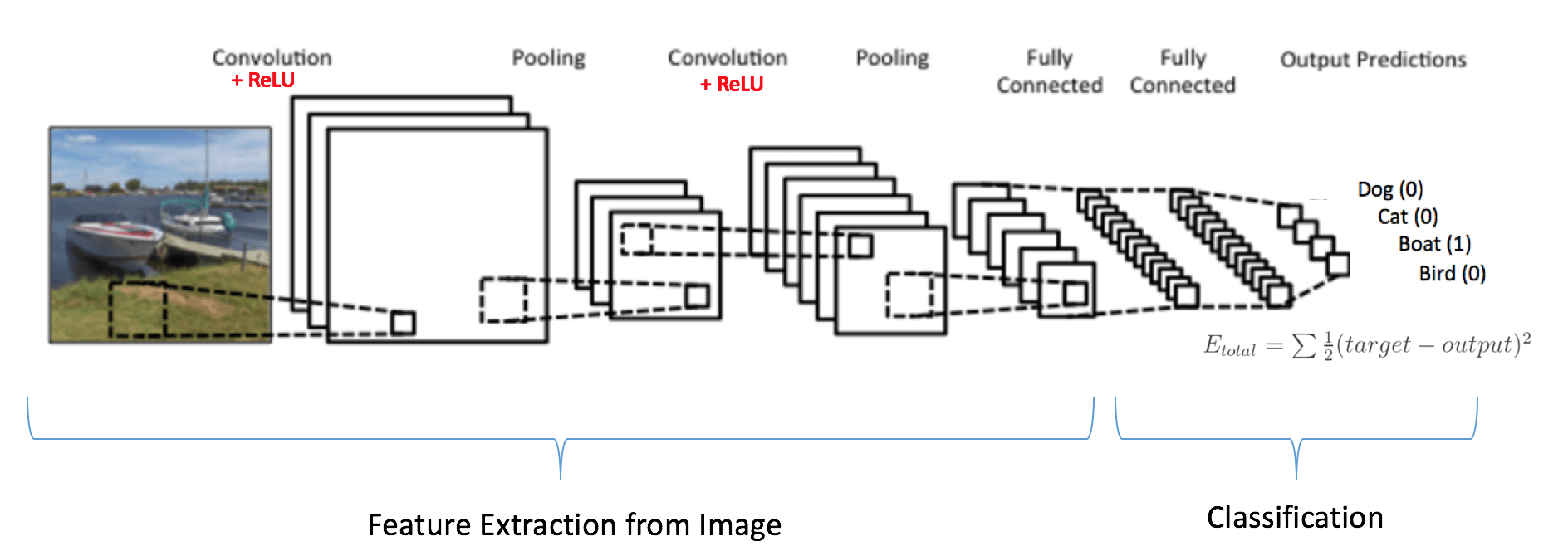
In this model, we will be using two layers of convolution filters and pooling operations. The first layer here consists of 32 3×3 filters. The second layer consists of 64 3×3 filters. The number of filters used here is selected randomly, and you can try experimenting with these values.
The pooling operation used in both these layers is 2×2 MaxPooling – it calculates the maximum value for every patch of the feature map and replaces the patch with that maximum value. A similar Convolutional Neural Networking design is shown in the following figure.
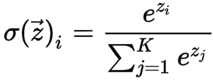
Furthermore, the dense neural network uses the relu activation function and consists of just a single layer of a dense network. The softmax activation function is implemented in the output layer, which predicts a multinomial probability distribution. The softmax function’s mathematical expression is shown below.
Creating a CNN Model in Python
Let’s begin creating and training our CNN model to classify CIFAR images using the Tensorflow library in python. First, set up Python in your system and install all the required libraries (tensorflow, matplotlib and numpy). This model is implemented in Google Colaboratory.
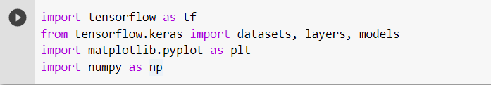
- Importing the required libraries
This tutorial will require three external libraries – tensorflow, numpy and matplotlib. The Keras sequential API is used from the tensorflow library, making it very convenient for creating and training the model with just a few commands. The numpy library is used for performing the mathematical computations while training the model.
The matplotlib library has been used for visually displaying the images of the dataset.
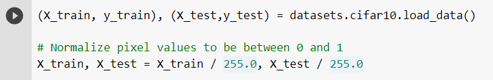
- Downloading and including the CIFAR10 dataset
We have already discussed the CIFAR10 dataset, which we will be using to train and test our model.
Using the following commands, download and include the dataset into your IDE or code editor.
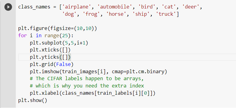
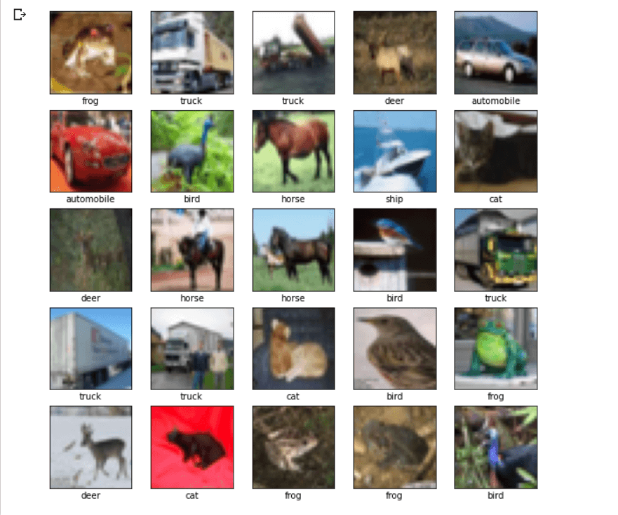
Let’s plot the first 25 images from the training set and show the class name underneath each image to make sure the dataset looks right.
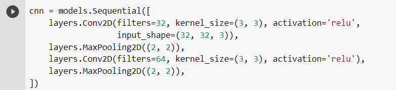
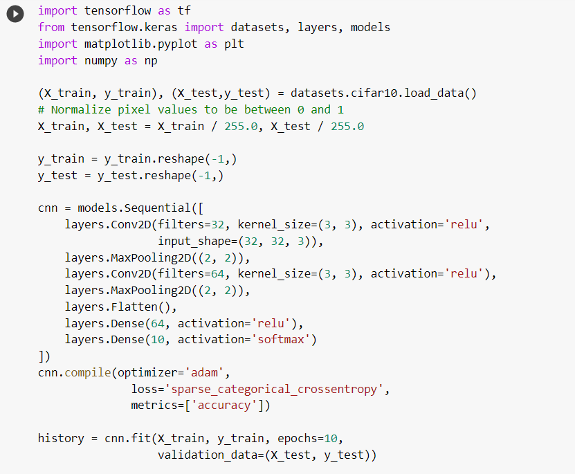
- Creating the Convolutional Base
Now we’ll create our model’s convolution base. Two layers of convolution filters and pooling operations are used. As input, the CNN takes tensors of shape (image_height, image_width, color_channels), ignoring the batch size. As our dataset has 32×32 images of 3 color channels (R,G,B), the tensor shape is : input_shape = (32, 32, 3).
The pooling operations used in the two layers are MaxPooling2D which calculates the maximum value for each patch of the feature map and replaces the patch with this maximum value.
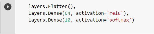
- Adding Dense Layers to the Model
For completing the model, the final output tensor from the convolutional base (of shape (4, 4, 64)) is fed into one or more Dense layers to perform classification. The dense layers take vector inputs, i.e. 1-dimensional arrays. Thus, before creating the dense layer, we flatten the y_train[] and y_test[] arrays into 1-dimensional arrays.
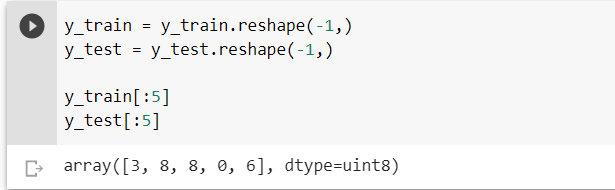
This flattened output is fed to a feed-forward neural network, and backpropagation is applied for training the model. The dense layer uses the softmax activation function at its output layer. The softmax function normalizes the probability summing up the two values to 1.
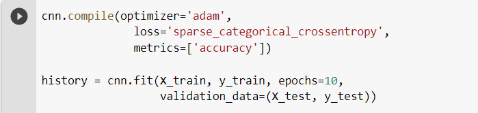
- Compiling and Training the Model
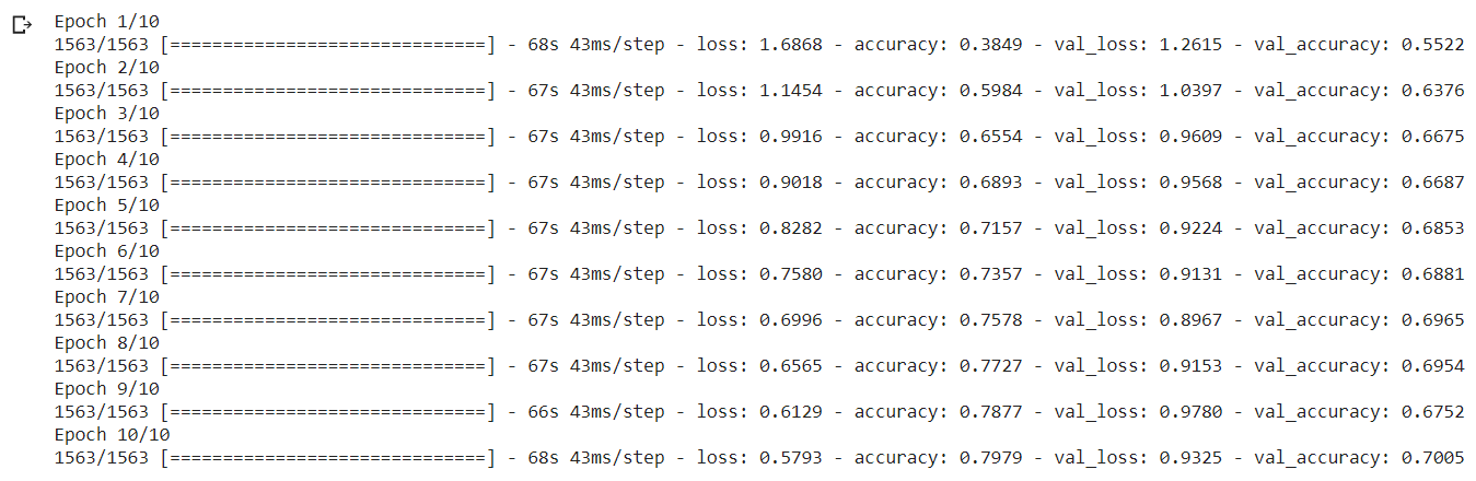
The following commands are used to compile and train the model. Here, we have used ten epochs for training the model, i.e. it will go through the entire dataset and check and improve errors in the predictions ten times or for ten iterations.
- Evaluating the Model
We can see that the model has a 70.05 percent accuracy, which is very high compared to other algorithms like ANN or RNN. It also takes less time because of the pooling operations, which reduce computing time.
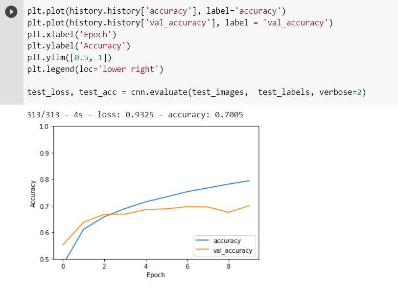
The gap between the test accuracy and validation accuracy indicates the degree of overfitting. Overfitting increases as the gap widens. When the model becomes extremely good at classifying or predicting data from the training set but not so good at classifying data it wasn’t trained on, we call this overfitting. In other words, the model has overfitted the training set data.
Final Output Predicting Some Images From The Dataset :
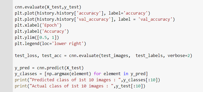 The output of the above code is shown below.
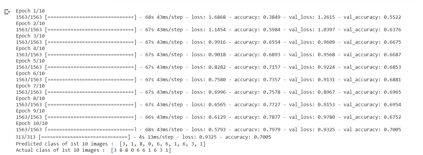 Here, the model predicted and classified the first ten images of the dataset as per their respective classes. We can observe that it classified nine images accurately, and one of the images (the 2nd image) was misclassified. But this is an excellent result for a model having around 70% accuracy.
Also Read: Why Python Is So Essential For Machine Learning?