Exploratory Data Analysis (EDA) is the crucial process of using summary statistics and graphical representations to perform preliminary investigations on data in order to uncover patterns, detect anomalies, test hypotheses, and verify assumptions.

In simple words, EDA is a data exploration technique to understand the various aspects of the data. EDA is often used to see what data may disclose outside of formal modelling and to learn more about the variables in a data collection and how they interact. It could also help us figure out if the statistical procedures we are considering for data analysis are appropriate. Before modelling the data, it gives insight into all of the data and the numerous interactions between the data elements.

Importance of EDA in Data Processing and Modelling 

EDA makes it simple to comprehend the structure of a dataset, making data modelling easier. The primary goal of EDA is to make data ‘clean’ implying that it should be devoid of redundancies. It aids in identifying incorrect data points so that they may be readily removed and the data cleaned. Furthermore, it aids us in comprehending the relationship between the variables, providing us with a broader view of the data and allowing us to expand on it by leveraging the relationship between the variables. It also aids in the evaluation of the dataset’s statistical measurements.

Outliers or abnormal occurrences in a dataset can have an impact on the accuracy of machine learning models. The dataset might also contain some missing or duplicate values. EDA may be used to eliminate or resolve all of the dataset’s undesirable qualities.

Data Cleaning and Preprocessing 

Data preprocessing and cleansing are critical components of EDA. Understanding the variables and the structure of the dataset is the initial stage in this process. The data must then be cleaned. The dataset may contain redundancy such as irregular data, missing values or outliers that may cause the model to overfit or underfit during training. Removing or resolving these redundancies is known as data cleaning. The last part is analysing the relationship between the variables. 

Performing EDA on a Sample Dataset

To further grasp EDA, we’ll look into a few instances.

Dataset used for Demonstration

For this demo, we will be using the dataset named “Students Performance in Exams” downloaded from Kaggle. 

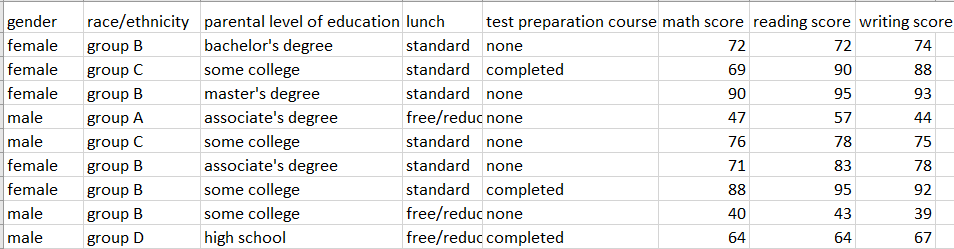
This dataset contains the following attributes :

1. Gender
2. Race/Ethnicity
3. Parental level of education
4. Lunch
5. Test preparation course 
6. Maths score
7. Reading score
8. Writing score

Importing Required Libraries and Reading the Dataset

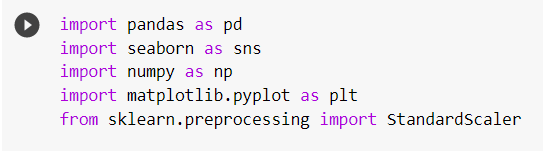
We will be using five external libraries for this demonstration.

1. Pandas – for reading the dataset files
2. Seaborn – for graphical visualization of the data
3. Numpy – for numerical calculations
4. Matplotlib – for graphic visualization 
5. Sklearn – for scaling the dataset

Next, we read the dataset using the pandas library. 

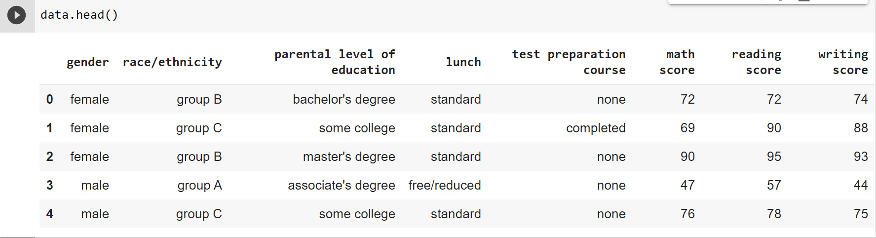
The first five and the last five elements of the dataset are displayed in the following code snippet using the head() and tail() methods, respectively. 

Cleaning the dataset

In data cleaning, we will cover the following operations. 

1. Checking and removing or resolving null/missing values
2. Dropping the columns which are not necessary for ML modelling
3. Checking for outliers in the dataset 
4. Normalizing and scaling the dataset values

Checking for null or missing values in the dataset

The info() method provides details about the dataset, such as the number of null values, data types, and memory utilisation.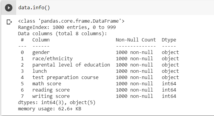

So, as you can see from the preceding code snippet, the dataset is free of any missing or null values.

The describe() method may also showcase some of the most relevant qualities of the dataset.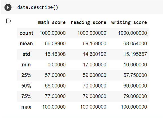

Even though the dataset has no missing values, suppose there are some null values in the dataset while building an actual ML model. These missing values can be dealt with in one of the following methods.

1. Replacing the null values with the mean values
2. Replacing the null values with the median values
3. Replacing the null values with the mode values
4. Dropping the values in case if the dataset is huge

If the dataset contains any outliers, the first three approaches are not recommended since they will alter the mean, median, and mode values.

Assume the ‘math score’ column in the dataset contains a null value. The median value now replaces the null value in this column. This code snippet for this operation is displayed below.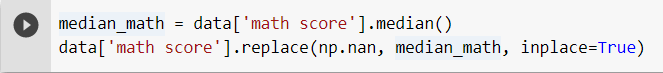

Removing Columns that ay not be Utilized for ML Modelling

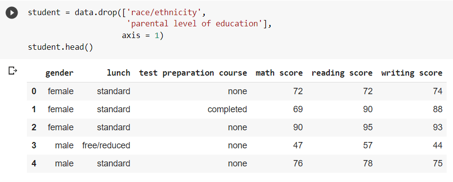
Assume that the columns ‘race/ethnicity and ‘parental level of education’ are unnecessary for a specific ML model. As a result, we remove the columns from the dataset that are not necessary.

Checking for outliers in the dataset

Outliers in a dataset are extreme results that can occur due to measurement variability, experimental mistakes or other factors. They can pose substantial issues in statistical analysis and significantly impact the performance of any machine learning model.

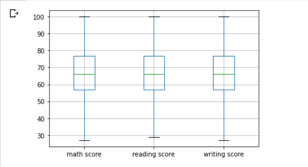
The Boxplot may be used to discover outliers in a dataset.

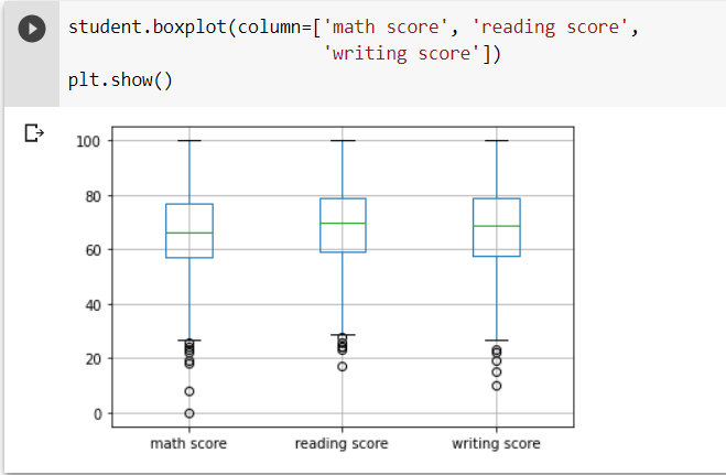
The standard values are present within the block, while the outliers are shown by the little circles outside the block, as can be seen above. Outliers can be omitted in big datasets, but because our sample is smaller, we will replace them with IQR (Interquartile Range Method).

The IQR is determined as the difference between the data’s 25th and 75th percentiles. By sorting the selected data at specific indices, the percentiles may be determined. By putting boundaries on sample values that are a factor k of the IQR, the IQR is utilised to identify outliers. The value 1.5 is a common value for the factor k.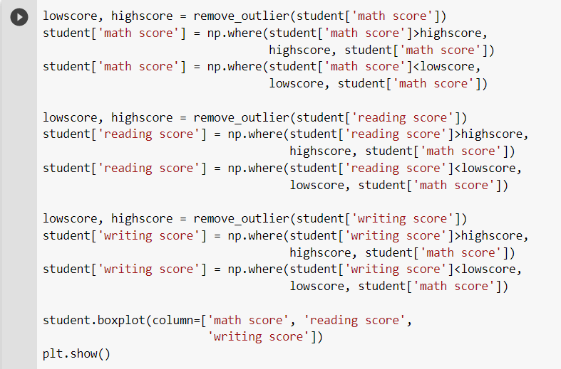

Data Normalization and Scaling of the Features

Data normalisation, also known as feature scaling, standardises a data set’s range of attributes, which might vary considerably. As we can see, the dataset comprises student grades ranging from 0 to 100, which is a pretty wide range. Scaling the features simplifies the computing processes involved in model training and improves accuracy. The StandardScaler() method from the sklearn package may be used to scale data.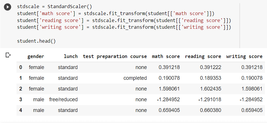 

Now that the data has been scaled down to a smaller range, it can be utilised to train machine learning models more easily.

Analysis of Relationship Between the Variables

It’s crucial to examine the relationship between variables to determine if they’re dependent or independent. It is critical to select the predictor variable while training any ML model. This can be done by plotting correlation matrices, scatter plots, histograms and other graphical analysis approaches. For our dataset, we’ll see a handful of them.

Plotting Pairwise Correlation using Heatmap

The heatmap displays the correlation between each variable on a scale of -1 to 1, with 1 denoting total positive correlation, 0 denoting no correlation, and -1 denoting absolute negative correlation.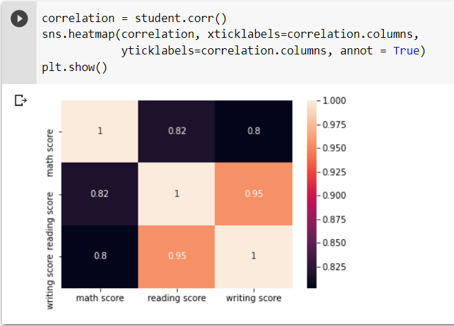

Since the three variables are all marks in various topics ranging from 0 to 100, they have a strong correlation.

Analysis Using Scatter Plot

The scatter plot aids in understanding the relationship between variables that are dependent on each other. The scatter plot between ‘math score’ and ‘reading score’ dependent on the type of ‘lunch’ the students had is shown in the following code snippet. 

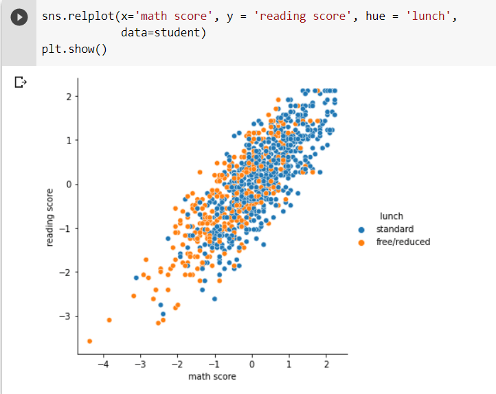
We may conclude from the scatter plot that children who ate standard lunch did better on reading and math examinations than children who ate free or reduced lunch.  

To explore the relationship between variables in a dataset. Our dataset is now ready to be utilized for training machine learning models, and we have a thorough understanding of it, allowing us to create suitable ML models.

Also Read: R Programming Series: Exploratory Data Analysis