

Time series forecasting is a hot topic with a wide range of applications including weather forecasting, stock market forecasting, resource allocation, business planning, and so on. We want to find Y(t+h) with the use of currently available data Y(t) in time series prediction. LSTM networks make it easy to make time-series predictions.
Let’s start with RNN and then move on to LSTM. RNNs are a type of Neural Network in which the previous step’s output is used as the current step’s input. Standard neural networks’ inputs and outputs are all independent of one another, but in certain cases, such as when predicting the next word of a sentence, the previous words are used, and therefore the previous words must be stored in memory.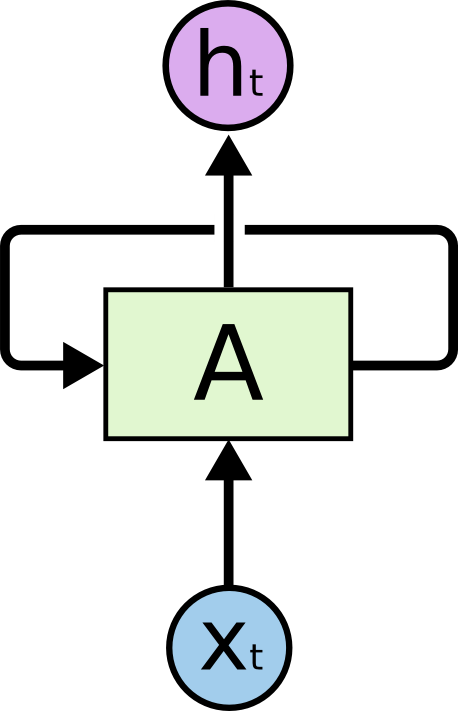
RNNs have memory, which ensures they can process or predict future outcomes based on previous outputs. RNNs, on the other hand, have a limited short-term memory that means they can only retain a limited amount of previous outputs. A vanishing gradient occurs as the effect of previous inputs fades and disappears with subsequent inputs, influencing the output. As a result, we must solve the RNN’s short-term memory dilemma in a model that requires recalling a greater volume of data in order to make predictions.
LSTM – Long Short Term Memory Networks
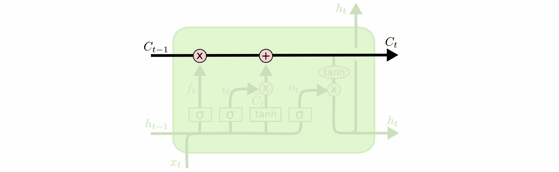
The LSTM, a special kind of RNN, solves the problem of short term memory in RNNs by adding a long term memory cell state.
Let us look at a scenario to help us understand. Consider a scenario where we want to use an LSTM model to predict the next few words in a sentence to save time and reduce effort while typing. Assume a user types “Ram likes to eat pizza, and his favourite cuisine is” and the model predicts the next word and immediately types “Italian.” The key term here is ‘pizza’. Since this keyword can be used to predict the cuisine, it must be stored or carried with all other inputs (in this case, other words of the sentence). As a result, the long-term memory cell will hold the input ‘pizza’ until the last part, i.e. the sentence’s last word. It has a forget gate that deletes previously-stored inputs, leaving only the inputs or keywords required for the next prediction in the long term memory cell. A long term memory cell state is shown in the figure below.
 This article will take you through a basic LSTM model that was created to forecast or predict potential bike-sharing in London based on historical records.
Dataset Used For Training and Testing The Model
The dataset named “London Bike Sharing Dataset” used for training and testing the model is downloaded from Kaggle. It contains hourly data of the count of people sharing the bikes along with all the weather parameters. 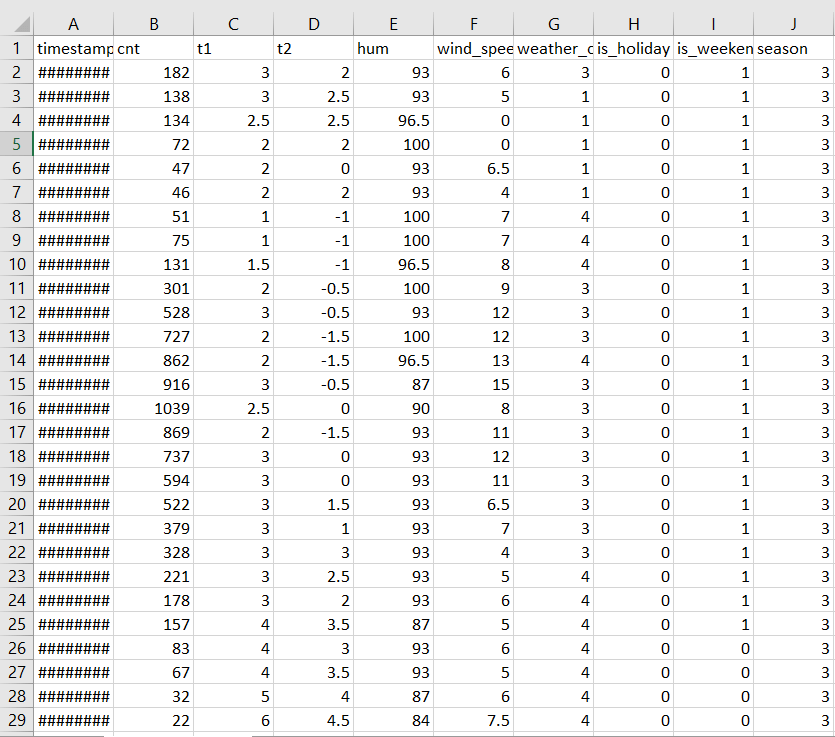
Implementation of the LSTM Time Series Prediction model in Python
Let’s begin creating a simple time series prediction system to predict future bike-sharing in London based on the data of bike-sharing in the past. First set up Python in your system and install all the required libraries (TensorFlow, matplotlib and numpy). This model is implemented in Google Colaboratory.
Importing required libraries:
This tutorial requires a few external libraries which are stated below. The Keras sequential API is used from the TensorFlow library, which makes it very convenient for creating and training the model with just a few commands. The numpy library is used for performing the mathematical computations while training the model.
The matplotlib library has been used for visually displaying the images of the dataset.The pandas library for reading the dataset file.The matplotlib library for graphically displaying the results obtained and sklearn for splitting the available dataset in order to use a part of the dataset as a training dataset and another part as a testing dataset. 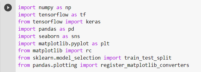
Downloading and loading the dataset:
The “London Bike Sharing” dataset can be downloaded in Google Colaboratory by using the command shown in the following code snippet. 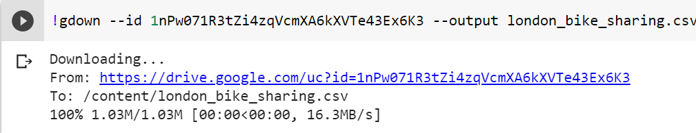 If we are using any other IDE or code editor, the datasheet can be downloaded from Kaggle. We load the dataset into a Pandas dataframe after downloading it.
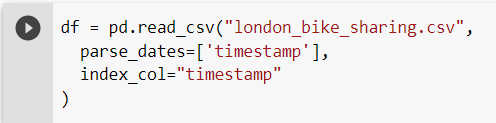
The timestamp strings are parsed as DateTime objects by pandas. We can just display a few records from the dataset for confirmation. 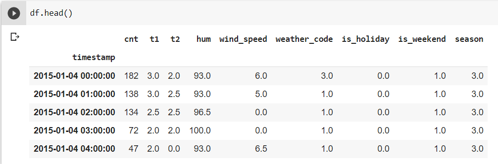 Scaling and other preprocessing of the dataset:
We’ll start by splitting the dataset into two sections: one for training the model and the other for testing it.
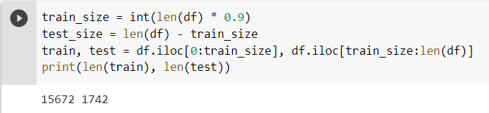 So, the training dataset now has around 15,000 samples and the test dataset has around 1,700 samples. Then we scale the data as scaling will reduce the computational time and it provides more accurate results. We have scaled the column ‘count’ (‘cnt’) along with the other features of the dataset.
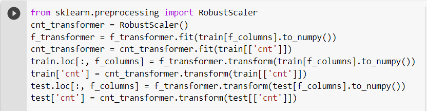
We must split the time series data into smaller sequences in order to use the dataset. We do this by writing a function called create a dataset() that takes the parameters X (i.e. features), y (i.e. labels) and the number of time steps we need to use as history for our sequence. The function returns the subsequences created. 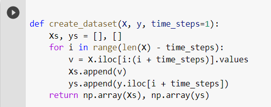 We set the time steps to 48, implying that the model would forecast future bike-sharing based on data from the previous 48 hours.
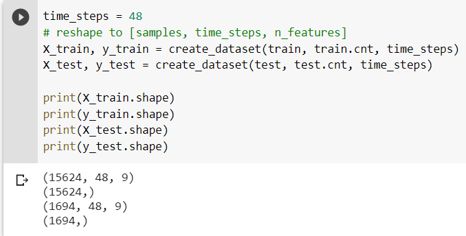 Creating the LSTM model:
Now we’ll use the Keras sequential API from the tensorflow library to construct our LSTM model.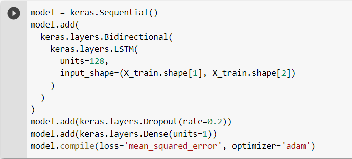 The Dropout layer, which helps avoid overfitting, sets input units to 0 at random with a rate of 20% at each stage during training of the model. We then use the training dataset to train the model.
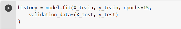 Evaluation and Testing of the Model:
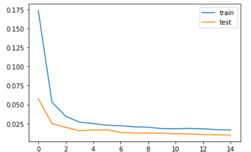
The model has been developed and is now able to make predictions. The separation between the two curves is very small in the plot of loss and validation loss, showing that there is no overfitting and the model is working well.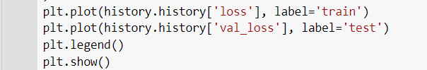
 Now, we make some time-series predictions using the model. As previously described, we used data from the previous two days to forecast bike-sharing in the coming days. To compare the results, we display the real test data and the expected test data in separate plots.
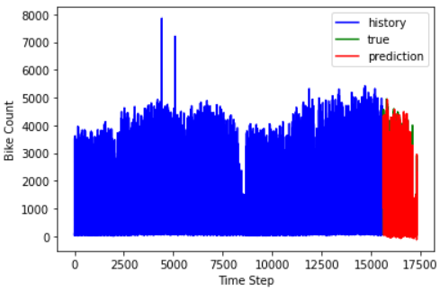
Here, the blue-coloured graph shows the training data, the green-coloured graph shows the actual test data and the red coloured graph shows the predicted data.
To evaluate more clearly, we plot them separately. 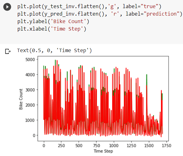
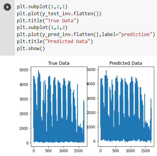
As we can observe that the actual test data and the predicted data are approximately identical. We can conclude that the model is efficient and performs time series predictions using LSTM with a good amount of accuracy.


 models. Read now in our latest article!)