Wherever you are as you read this blog, I want you to take a moment and think back to how you went about your day, every small decision you consciously and unconsciously made, to get to where you are right now.
Perhaps, just like every student ever, you got caught up in assignments till late last night and could barely make it to the last bus leaving for your college that’d just about get you to class in time were it not for your mother who screamed, “IT’S ALREADY 8:00 A.M YOUR CLASS STARTS IN 20 MINUTES!”, jolting you back to reality.
Or maybe you’re a working professional and your boss declared, “It’s a slow day at work today fellas” so you’re just looking to brush up on your Deep Learning skills on the side.
Or maybe you’re a hobbyist, just here for the fun of it.
Whatever the case may be, and however you got to read this blog today, I want you to think if you would still be here reading and understanding any of this if:
i. You could see everything but without the ability to interpret what you see.
ii. You could hear everything around you but without the ability to understand any language at all.
That seems quite harsh. But clearly, the answer is no.
You wouldn’t get out of bed if your brain hadn’t interpreted whatever your mother yelled about it being 8:00 a.m and your class starting in 20, because you obviously wouldn’t know what any of that means or why that is a problem. For you, it would just be incongruous noise.
You wouldn’t have made the decision to browse Deep Learning concepts if it weren’t for you understanding what, “a slow day at work” means.
In, the same manner you wouldn’t be able to read or process any word of this blog because your brain wouldn’t know what a ‘word’ is in the first place.
All your brain would see is white, with some black interspersed.
You see, interpreting what you see, and what you hear, is something that we take for granted but cannot possibly survive without.
It’s the same with a machine.
In our previous two blogs, Deep Neural Networks with Keras and Convolutional Neural Networks with Keras, we explored the idea of interpreting what a machine sees. With this blog, we move on to the next idea on the list, that is, interpreting what a machine hears.
In the Deep Learning world, we have a fancy term for this. We call it, Natural Language Processing.
To learn more about Deep Learning, you can try out the “Practical Deep Learning with Keras and Python” online tutorial. The course comes with 3.5 hours of video that covers 8 vital sections. These include theory, installation, case studies, CNN, Graph-based models and so much more! This course is especially a helpful tool mainly if you are a beginner.
Also, you can opt for a similar online tutorial “The Deep Learning Masterclass: Classify Images with Keras”. Like the above, this course requires no prior experience either. The tutorial brings you videos of 6 hours where it covers 7 impressive topics that are important in understanding the concept deeper.
Natural Language Processing includes text processing (like the words in this blog), audio and speech processing.
Before we discuss how we can enable a machine to interpret speech or process text, we need to understand some concepts. I recommend you go through our previous blogs in this series for a seamless read.
Right.
Consider a sentence from this blog itself.
“In the Deep Learning world, we have a fancy term for this. We call it, Natural Language Processing.
Natural Language Processing includes text processing (like the words in this blog), audio, and speech processing.”
Now consider this modified sentence and note how it will still make absolutely perfect sense to you,
“In the Deep Learning world, we have a fancy term for this. We call it, Natural Language Processing.
It includes text processing (like the words in this blog), audio and speech processing.”
The difference, of course, is just that I replaced Natural Language Processing with an ’It’.
What do we learn from this? We learn that we interpret subsequent words based on our understanding of previous words.
We could immediately understand that ‘It’ refers to Natural Language Processing.
We don’t read one word, throw everything away, and then read another word and start thinking from scratch again.
Our thoughts have persistence.
For example, if you are developing an application that requires you to automatically calculate player runs in a game of cricket from the live telecast, you would first need your application to judge how many runs were scored (whether it was a 4 or 6 or a single) and then you would need to have the context from previous frames that would tell you WHICH PLAYER scored those runs so that you can add that many runs to the total for THAT PLAYER. It is difficult to imagine a conventional Deep Neural Network or even a Convolutional Neural Network could do this.
This brings us to the concept of Recurrent Neural Networks.

In the above diagram, a unit of Recurrent Neural Network, A, which consists of a single layer activation as shown below looks at some input Xt and outputs a value Ht.
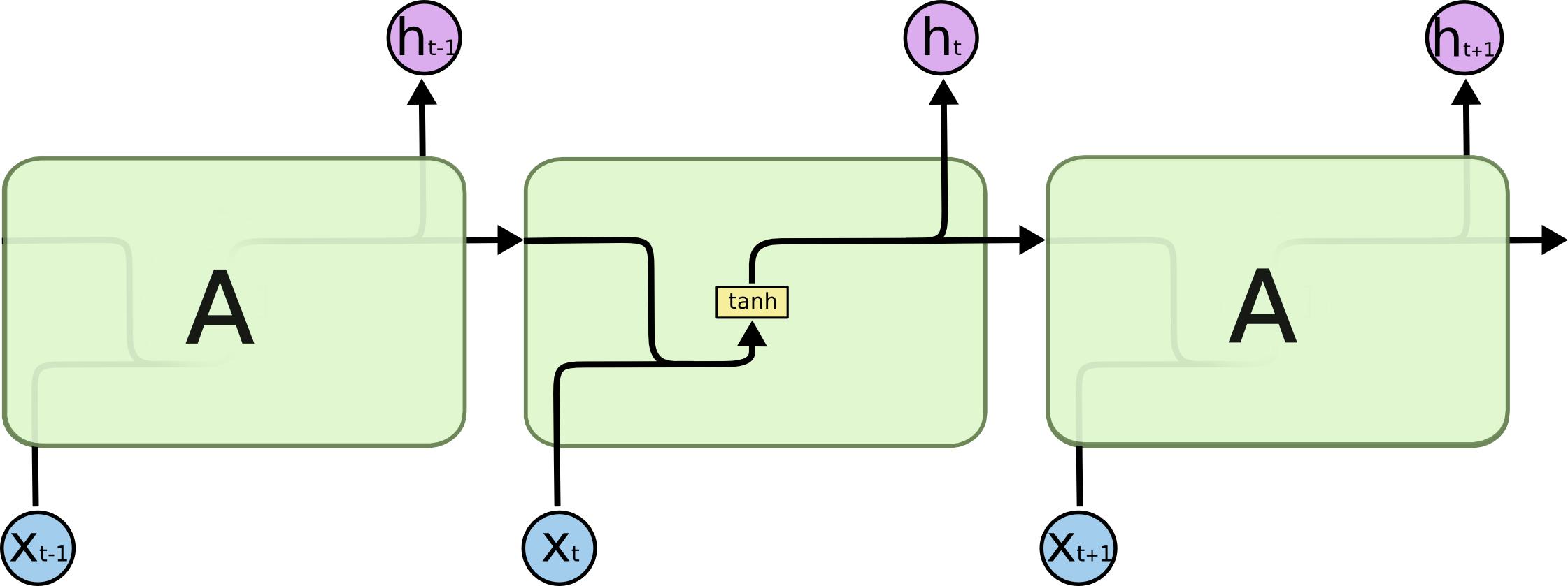
A loop allows information to be passed from one step of the network to the next. When we ‘unroll’ this loop architecture, we can see that basically, each unit passes a message to a successor, like a sequence.
Past inputs, thus influences decisions made on the present outputs.
This is the key that was missing.
When the network begins to see things as ‘sequences’, we can immediately see that this solves our network’s initial problem of retaining or understanding ‘context’.
A question then, which should crop up in your mind is, from how far back in the sequence can a Recurrent Neural Network hold a context?
To reframe this, the question in focus is from how far back can past inputs, Xt, still influence the outcome of the present input activations Ht?
Well, unfortunately, not so far back. But let’s understand everything with example because we believe examples are the best way to learn.
Consider, we are trying to predict the last word in “when birds flap their wings they …”, we don’t need any further context, it’s pretty obvious that the next word is going to be fly. In such cases, where the gap between the relevant information and the place that it’s needed is small, Recurrent Neural Networks can learn to use past information.
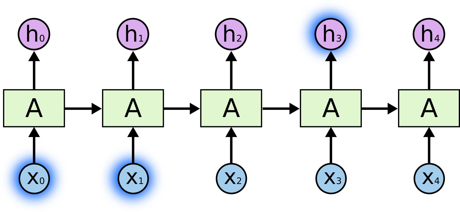
But if you consider a sentence as complex as the one we took as our example at the very beginning,
“In the Deep Learning world, we have a fancy term for this. We call it, Natural Language Processing. It includes text processing (like the words in this blog), audio and speech processing.”
Now if we were to predict the word after ‘and’ in the sentence above, we would first need to know what ‘It’ refers to.
For this, we have to go even further back.
It’s entirely possible for the gap between the relevant information and the point where it is needed to become very large as in our example.
Unfortunately, as that gap grows, Recurrent Neural Networks become unable to learn to connect the information.
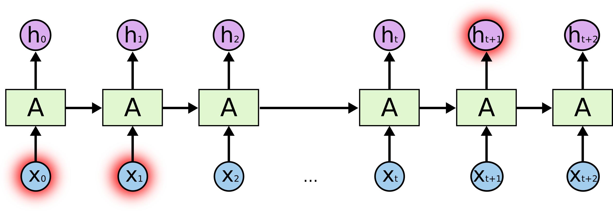
This is why we need LSTMs. Because LSTM units are perfectly capable of ‘remembering’ long term dependencies in a given sequence. In fact, LSTM stands for Long Short Term Memory.
Of course, to achieve this complex behavior of being able to ‘remember’ context in ‘memory’, an LSTM unit also looks quite overwhelming in comparison to our Recurrent Neural Network.
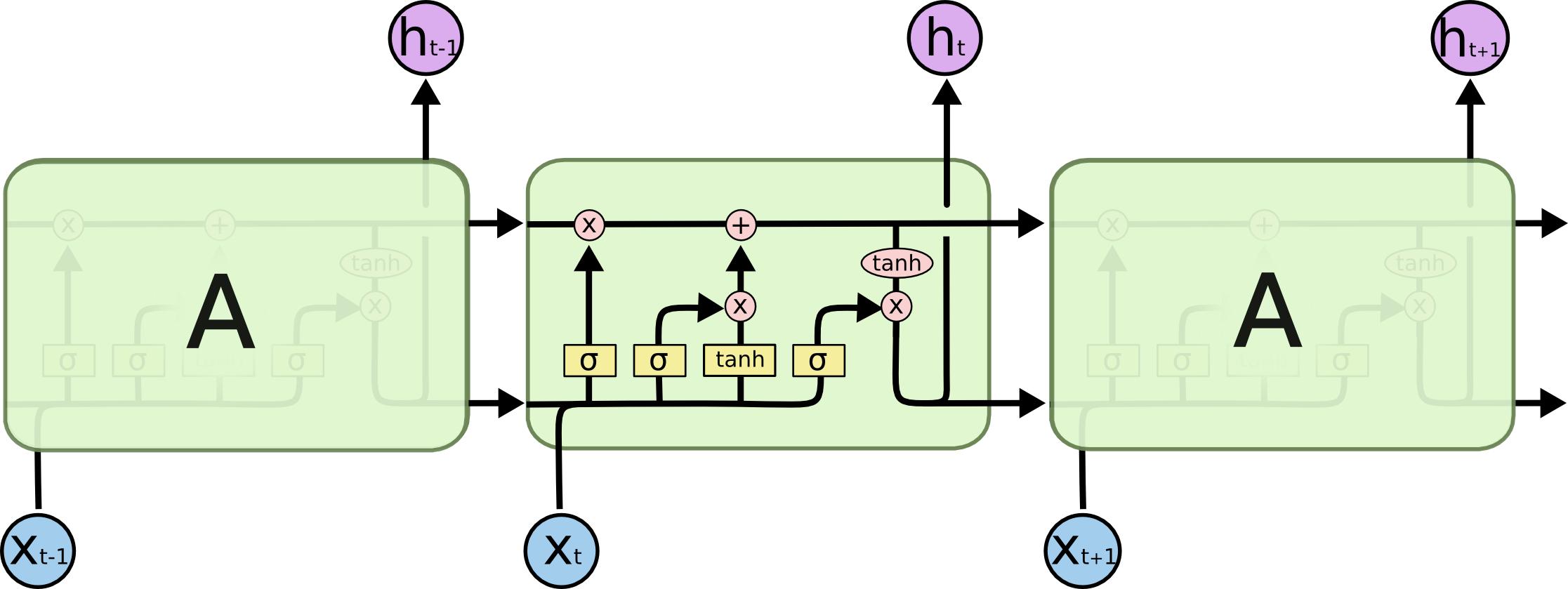
The mathematical details are beyond the scope of this tutorial. A more detailed explanation of LSTMs will be covered in the coming blogs.
For now, let us move on to the final and the most interesting part of this blog, the implementation.
Implementation of LSTM with Keras
For this tutorial blog, we will be solving a gender classification problem by feeding our implemented LSTM network with sequences of features extracted from male and female voices and training the network to predict whether a previously unheard voice by the network is male or female.
Step 1: Acquire the Data
The data for this tutorial can be downloaded from here.
Step 2: About the Data
After downloading the data, which should be about 1.4 GB, you will notice 4 folders inside labeled:
i. Male: Contains 3971 male audio files from different speakers (Male Training Set)
ii. Female: Contains 3971 female audio files from different speakers (Female Training Set)
iii. Male Test: Contains 113 male test audio from different speakers (Male Test Set)
iv. Female Test: Contains 113 female test audio from different speakers (Female Test Set)
The average duration of all audio files is about 5.3 seconds.
Step 3: Extracting Features from Audio (Optional)
Audio files are also one long sequence of numbers. But this sequence tends to be extremely long, almost 40,000 sequence numbers long, and because of our limited RAMs, we need to find more efficient ways to represent this sequence (audio).
This is done by extracting the pitch of the audio along with something called the Mel Frequency Cepstral Coefficients (MFCCs) of the audio which is just a mathematical transformation to give the audio a more compact representation.
Because we are dealing with audio here, we will need some extra libraries from our usual imports:
import numpy as np
import librosa
import os
import pandas as pd
import scipy.io.wavfile as wav
In case this throws you an import error, run the following line in your command prompt:
pip install librosa
pip install scipy
Next, specify the paths of the Male and Female folders ON YOUR MACHINE in the variables accordingly:
path_male = “C:\\Users\\Bhargav Desai\\Documents\\GitHub\\gender-classifier-using-voice\\Data Preprocessing\\Male\\”;

path_female = “C:\\Users\\Bhargav Desai\\Documents\\GitHub\\gender-classifier-using-voice\\Data Preprocessing\\Female\\”;


mfcc_col=[‘mfcc’+ str(i) for i in list(range(110))];

def main(path,gender):
df = pd.DataFrame()
print(‘Extracting features for ‘+gender)
directory=os.listdir(path)
for wav_file in directory:
write_features=[]
y, sr = librosa.load(path+wav_file)
fs,x = wav.read(path+wav_file)
print(wav_file)
mfcc_features=get_mfcc(y,sr)
write_features=[pitch]+mfcc_features.tolist()[0]+[gender]
df = df.append([write_features])
df.columns = col
df.to_csv(gender+’_features.csv’)


def get_mfcc(y,sr):
y = librosa.resample(y, sr, 8000);
y = y[0:40000];
y = np.concatenate((y, [0]* (40000 - y.shape[0])), axis=0);
mfcc=librosa.feature.mfcc(y=y, sr=sr, n_mfcc=10,hop_length=4000);
mfcc_feature=np.reshape(mfcc, (1,110))
return mfcc_feature


main(path_male,’Male’)
main(path_female,’Female’)
Although this part seems complicated, do not worry. It is okay if you do not understand this part of the code.
It is completely okay to skip this part for now.
All you need to remember is that this part of the code gives you a compact representation of the audio sequence for both the genders.
The outcome of this should be two .csv files named male_features.csv and female_features.csv in the same directory containing a compact representation of our audio sequences where each sequence is of length 113!
Consequently, we have successfully reduced our audio sequence length from 40,000 to 113!
In case you encounter compatibility errors, please comment on your errors down below or directly download the feature extracted .csv files by clicking here.
Step 4: Labelling & Preparing the Data for LSTM Model
The outcome of the previous step was that we got compact representations of male and female audio sequences which might give you the impression that the data is ready.
However, we are missing one critical element: Labels.
Before we can train, we need to label our data so that our network can learn the difference between males and females from our data.
We do this by first loading our data from the two .csv files we have obtained:
os.chdir(‘/Users/bhargavdesai/Downloads’)
maledf = pd.read_csv(‘male_features.csv’)
femaledf = pd.read_csv(‘female_features.csv’)
NOTE: Make sure that you pass the directory/folder where you have downloaded the .csv files from the above link in the argument to os.chdir()
The output should look something like this:
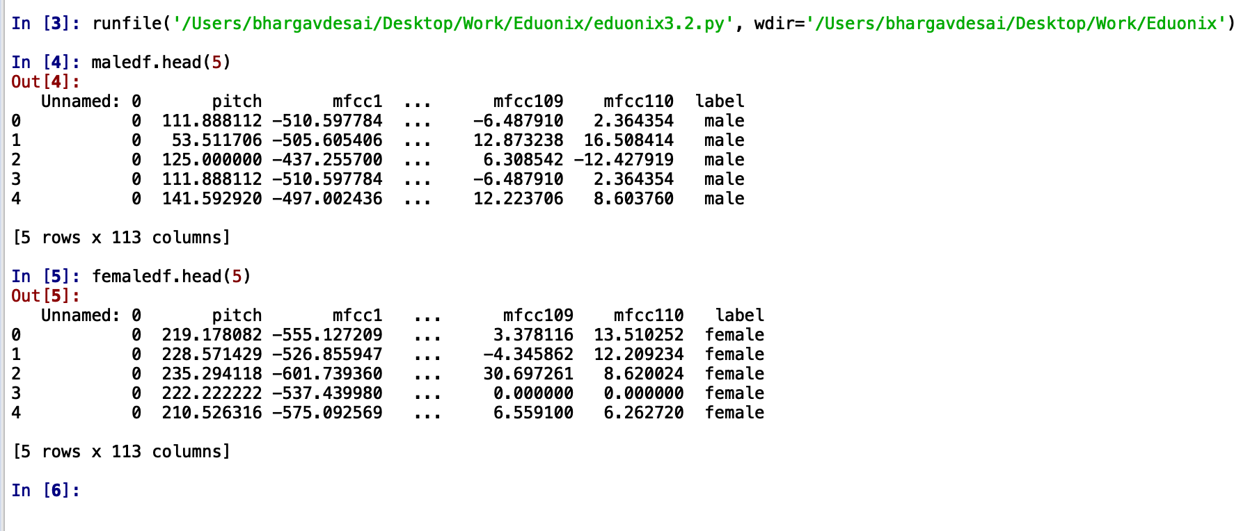
We can see that the label is ‘male’ or ‘female’ which is not in the form that we want.
We need to change this to a numeric form which is either ‘1’ or ‘0’
Here’s how we do it:
maledf.replace(to_replace=’male’, value=1)
femaledf.replace(to_replace=’female’, value=0)
You will have something like this printed out:
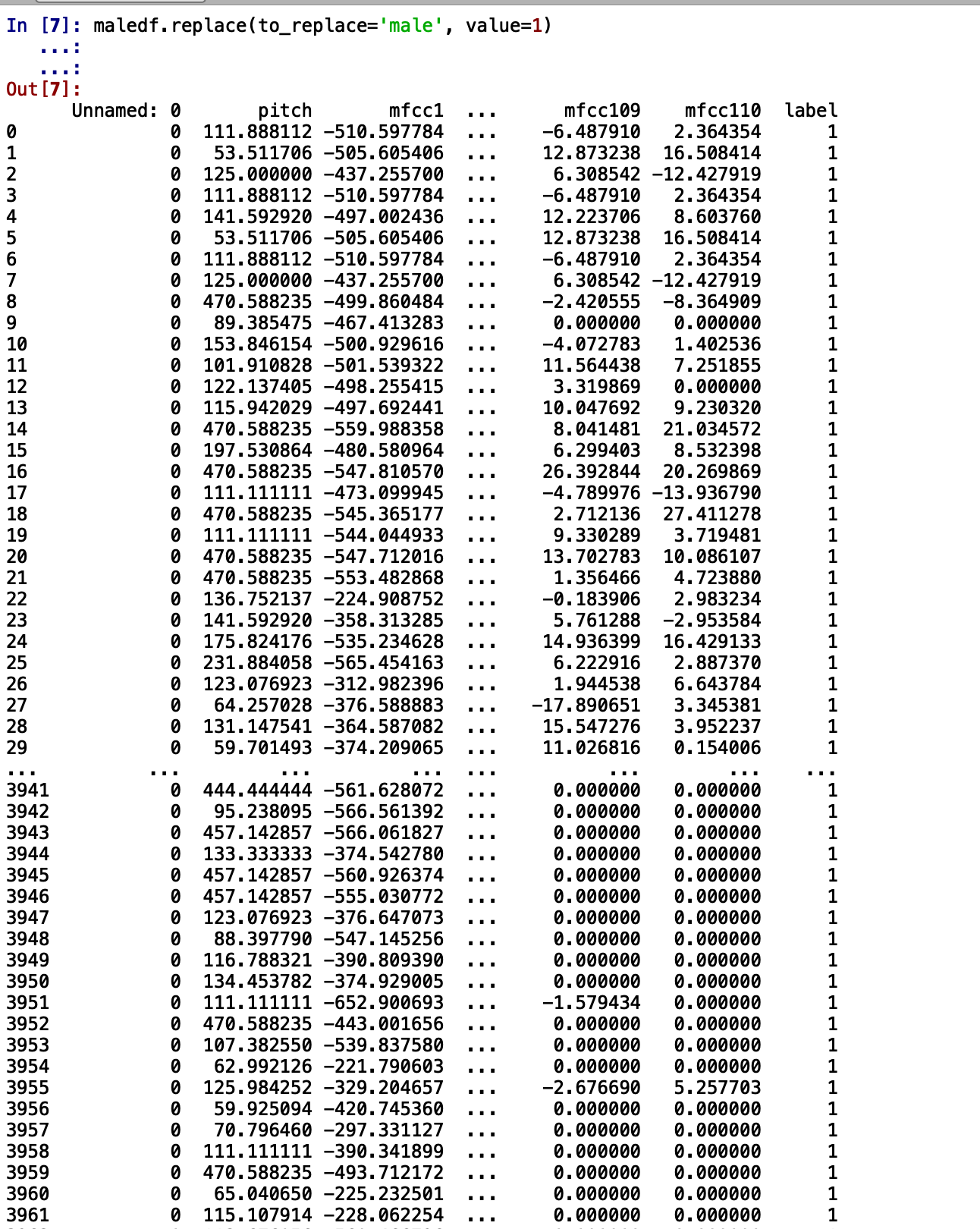
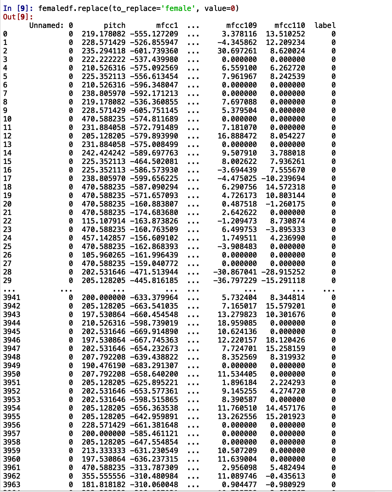 We can see that ‘male’ has been replaced by ‘1’ and ‘female’ has been replaced by ‘0’
We will now split it into our standard X_Train and Y_Train variable format so that we are consistent with the other blogs in this Keras series:
Male = maledf.replace(to_replace=’male’, value=1)
Female = femaledf.replace(to_replace=’female’, value=0)
X = pd.concat([Male, Female])
XTrain = X.sample(frac=1)
YTrain = XTrain[‘label’]
XTrain = XTrain.drop(columns="label")
X_Train = XTrain.values
Y_Train = YTrain.values
The pd.concat() function joins two DataFrames, X.sample(frac=1) randomly shuffles the rows of the joined DataFrame and the XTrain.values function converts the DataFrame to a Numpy array X_Train.
Note: Here X_Train is our training set and Y_Train are the labels that we separated using the XTrain[‘label’] function.
Step 5: Building an LSTM Keras Model
We have come to the conclusion of this blog where we will show you how to create an LSTM model to train on the dataset we have created.
We are now familiar with the Keras imports and Keras syntax. But we’ll quickly go over those:
The imports:
from keras.models import Model
from keras.models import Sequential, load_model
from keras.layers.core import Dense, Activation, LSTM
from keras.utils import np_utils
Then we create a Keras Model object by:
model = Sequential()
Then we can assemble our Keras LSTM model by:
model.add(LSTM(32, return_sequences=True, input_shape=(112, 1)))
model.add(LSTM(6, return_sequences=True))
model.add(LSTM(8, return_sequences=False))
model.add(Dense(1, activation = ‘sigmoid’))
model.compile(optimizer = ‘adam’, loss = ‘binary_crossentropy’, metrics=[‘accuracy’])
model.summary()
model.fit(X_Train, Y_Train, epochs = 20, batch_size = 32)
As soon as you run this code, you will get an error.
The error will read:
ValueError: Error when checking model input: expected lstm_1_input to have 3 dimensions, but got array with shape (7942, 112)
This happens because of the LSTM implementation in Keras expects sequences from you as input. A sequence has an additional dimension of ‘time’ in addition to the number of samples and features that are called ‘timesteps’ in Keras.
To rectify the error, just add this line of code before you start building the model:
X_Train = np.reshape(X_Train,(7942, 112, 1))
Here, our number of ‘timesteps’ which is basically how long our sequence is in time is equal to 112 with the number of samples 7942.
The result of running the code after the modification will show you a screen like this:
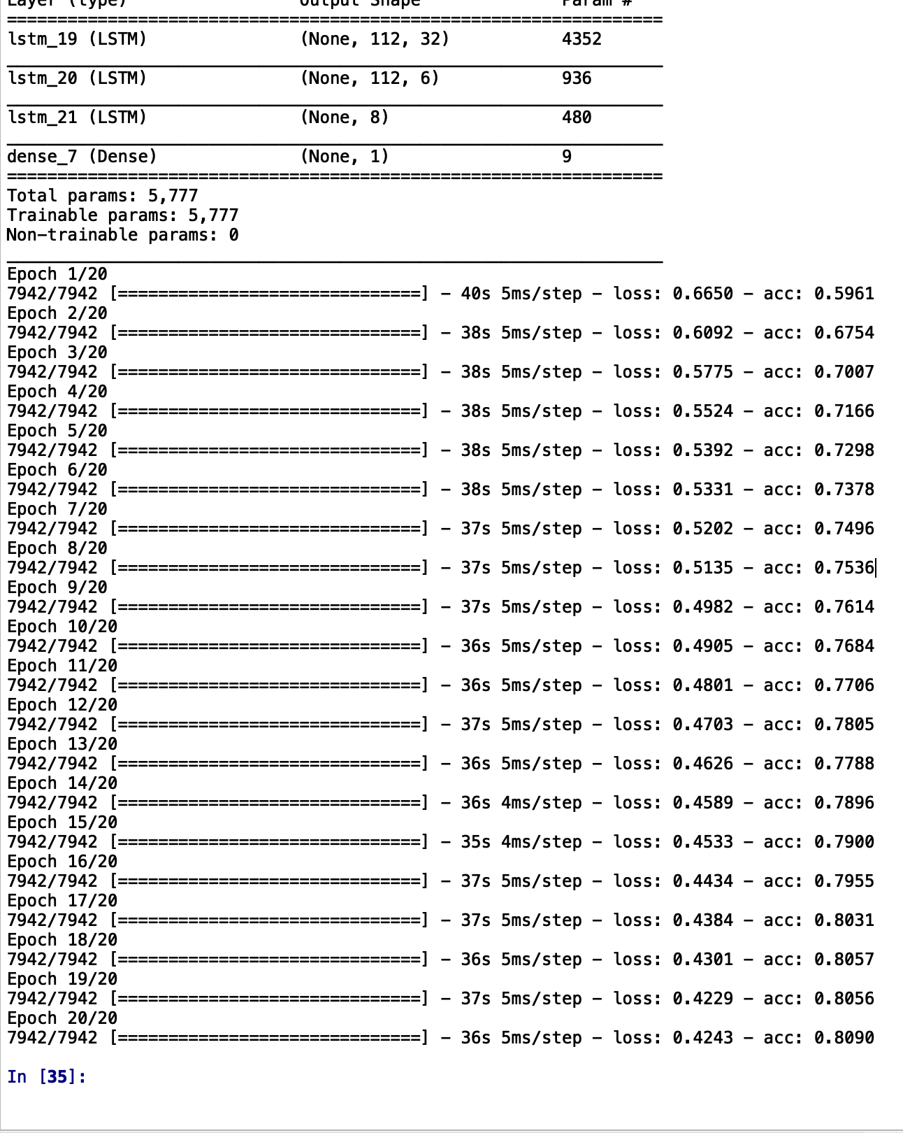 It can be seen that the accuracy is increasing consistently (~81% in just 20 epochs!) and the loss is also going down.
This indicates that our LSTM network is indeed learning how to differentiate between a male voice and a female voice!
On a concluding note from our side, we’d like to ask our inquisitive readers to see how much the accuracy goes up by when you train it for more epochs. At Eduonix, we push our students to go that extra mile so we’d also like to encourage all our readers here to see if they can use the code used in this tutorial to record their own audio and see if they can get our model to predict your gender correctly!

