

The Why and The How
In our previous blogs in the Keras series, we have explored Deep Neural Networks, Convolutional Neural Networks and Recurrent Neural Networks with LSTM. These ‘types’ of a Neural Network, as we’ve come to learn, are nothing but model architectures that are suited to their own domain of use. To know about these topics, you can refer the links given at the end of the article.
For a Convolutional Neural Network, the domain is images.
Hence, Convolutional Neural Networks are used for Computer Vision tasks.
For a Recurrent Neural Network, the domain is sequences which may be plain numbers, text, audio, or speech.
Hence, Recurrent Neural Networks come in handy for Natural Language Processing.

If we’re being honest about it, those are pretty much the most used terms that get thrown around in this part of the world.
And if we’ve covered the concepts and implementations of each, what is it exactly that warrants this blog?
That is the first and foremost thing we want to answer with this blog.
Because even though it might seem that we’ve pretty much exhausted Keras and Deep-Learning, it is also where we would be absolutely and profoundly, incorrect.
Artificial Intelligence and especially Deep Learning is a highly iterative field today. It is exceedingly rare, even for seasoned Data Scientists and Machine Learning Engineers, to develop an optimum model in their first attempt. The journey from suboptimal to optimality is the real test of anybody developing an AI solution.
To learn more about Deep Learning, you can try out the “Practical Deep Learning with Keras and Python” online tutorial. The course comes with 3.5 hours of video that covers 8 vital sections. These include theory, installation, case studies, CNN, Graph-based models and so much more! This course is especially a helpful tool mainly if you are a beginner.
The first course of preliminary or ‘first aid’ steps when the model you’ve trained does not meet expectations of optimality in terms of the loss of accuracy or any other metric would be to do the following:
1. Add more layers, more units.
2. Train for an increasing number of epochs
If the loss goes down significantly or if the accuracy seems to be increasing considerably, the answer to optimality is probably in a permutation somewhere there. We will shortly be publishing a more detailed and elucidated blog regarding these ‘first aid’ steps but the real problem is when these steps do not seem to be working at all.
This is what this blog is for.
A very predominant mistake that people make is in thinking that Artificial Intelligence is solely about how ‘intelligent’ you can get a machine to function or complete a particular task.
What’s not said enough, is that it’s not just about getting a machine to be ‘intelligent’, it is also equally important to be creative about how you teach the machine to be so.
Adding layers and layers, training for hours and days on end is not always a panacea.
So, what exactly do we mean by this? Where does the entire case for creativity come from?
Luckily, you’re at an Eduonix blog, and we teach with examples.
Let’s get to the problem then together and we’ll try to solve it with our knowledge of the previous blogs in the Keras series. The Convolutional Neural Networks with Keras blog in particular, since we are about to take up a Computer Vision example.
More From The Keras Series:
- Deep Neural Networks with Keras
- Convolutional Neural Networks with Keras
- Recurrent Neural Networks and LSTMs with Keras
Problem Statement
Given a set of shaky (motion blurred) images taken from a GoPro camera, we are to develop an Artificial Intelligence solution to sharpen the image.
Data
The data for this can be downloaded by the given link below:
https://drive.google.com/file/d/1H0PIXvJH4c40pk7ou6nAwoxuR4Qh_Sa2/view
The data has over 8000 images of resolution 1280×720 which makes it a heavy download but we encourage everyone reading this blog post, enthusiast or otherwise to download it and code along with us especially because automatic image de-blurring or sharpening is under rigorous research scrutiny and there is nothing better to sharpen your skills in Artificial Intelligence like a research problem.
Exploring the Data
Once the data has been downloaded, it needs to be unzipped. After you’ve unzipped it, save it to a convenient location.
From our previous knowledge of a Convolutional Neural Network or a Neural Network in general, we know that for it to learn anything useful we need to have two things:
1. Training Data
2. Labels for the Training Data
If you were to open the unzipped folder, you will notice two folders:
1. ‘train’
2. ‘test’

Open the ‘train’ folder and you will see 22 sub-folders with the naming convention as ‘GOPROabc_wx_yz’.

Each of these folders has yet another 3 sub-folders and a text document that can be neglected:
1. blur
2. blur_gamma
3. sharp
4. frames xx offset

Each ‘blur’ folder has approximately 50 odd motion-blurred images and the ‘sharp’ folder has the same images but sharpened.
The problem statement is to go from a blurred image to a sharp one.

It follows then, that this ‘blur’ sub-folder in each of the 22 sub-folders will have to be our training images and that our labels should be the images in the ‘sharp’ folder in each of those 22 sub-folders.
The testing data can be similarly located in the ‘test’ folder with exactly the same format.
We have thus explored and established our training and testing data.
(The ‘blur_gamma’ folder is exactly the same as the ‘blur’ folder with exactly the same images but with a further Gaussian blur over the motion blur. So we will exclude that folder from our discussion)
Alright then, let’s get coding everybody.
Loading the Data
The one problem with loading the data is that as mentioned earlier, each image has a resolution of 1280×720.
We have a total of 2100 blurred images (training data). Each image occupying almost 1MB on average. So to hold 2000 of those images, we will need over 2GB of RAM and then to run computations on those images we will exhaust even more RAM. Chances are, even if you have a 16GB RAM machine, it might crash. So to get around it, while loading the images in our memory while running the code, we will resize the image by using the cv2.resize() function of OpenCV library in Python. If this library is not installed on your machine, run the following on your terminal or command prompt:
pip install opencv (UNIX and Linux)
python -m pip install opencv-python (Windows)
Or if you have Anaconda installed on your machine (which we highly recommend) just type in:
conda install -c conda-forge opencv
Now, let us get to loading the data.
We will import the basic and necessary libraries along with OpenCV first:
import os
import cv2
import numpy as np
Now since we need to access the file system on your machine, we use the ‘os’ module of Python. This enables us to do things like open a folder or a sub-folder in that folder in running code etc.
Since we need to load the images into memory as arrays to work with them from where they are stored, it is intuitive why we may need the ‘os’ module.
We will first define the path to our ‘train’ folder since both our training data (blurred images), as well as their labels (, sharpened images) are in the ‘train’ folder.
path = ‘/Users/bhargavdesai/Downloads/GOPRO_Large/train’
Now we need to access the ‘blur’ folder in each of the 22 sub-folders in the ‘train’ folder to load all the blur images.
For this, we use the ‘os’ module.
The os.listdir() method lists all the folders present in the path passed as arguments and the os.path.join() just performs a join of the two strings passed as arguments with a ‘/‘ in between them.
The code for accessing each blurred image in each of the 22 subfolders can be written as:
appended_x=[] //create an intermediate empty list
X_train=[] //create an empty list for holding blurred images arrays

for folder in os.listdir(path_blur): //access each folder in ‘train’
for blur in os.listdir(os.path.join(path_blur,folder,’blur’)): //access the ‘blur’ sub-folder in each of the sub-folders in ‘train’
try:
c_blur = cv2.imread(os.path.join(path_blur,folder,’blur’,blur), -1) //load the images in a particular ‘blur’ folder
c_blur = cv2.resize(c_blur,(128,72)) //resize the image to make computations faster
X_train.append((c_blur))
print(“appended”+" “+blur+folder)
appended_x.append(blur+folder)
print(c_blur.shape)
except RuntimeError: //enter these red highlighted code lines ONLY for Mac users.
print(“.DS_Store file detected and dismissed”)
pass
X_train = np.asarray(X_train) //convert the list of images as array of images
Now we have all blurred images stored as a numpy array in the variable X_train.
If you remember from the previous blog, we need to scale the images to be between [0,1] since the neural activations only fire in that range and image are of the range [0,255].
X_train = X_train/255.0
print(X_train.shape)
The final shape should be: (2103, 128, 72, 3)
Similarly, we make an array for all the sharpened images following the exact same procedure:
Y_train=[]
appended_y=[]
for folder in os.listdir(path_sharp):
for sharp in os.listdir(os.path.join(path_sharp,folder,’sharp’)):
try:
c_sharp = cv2.imread(os.path.join(path_sharp,folder,’sharp’,sharp), -1)
c_sharp = cv2.resize(c_sharp,(128,72))
Y_train.append((c_sharp))
print(“appended”+" “+sharp+folder)
appended_y.append(sharp+folder)
print(c_sharp.shape)
except RuntimeError:
print(“.DS_Store file detected and dismissed”)
pass
Y_train = np.asarray(Y_train)
Y_train = Y_train/255.0
print(Y_train.shape)
The shape should be (2103, 128, 72, 3)
Now we have the training data and the labels, ready to go.
Let’s get to building the model:
Building the Model
First, we import the necessary:
from keras.models import Sequential
from keras.backend import tensorflow_backend as K
from keras.models import Model
from keras.layers import Input, Conv2D
from keras.optimizers import Adam
As we’ve learned from the previous blog, we first instantiate a Model object by the following line:
model = Sequential()

#add model layers
model.add(Conv2D(64, (3,3), activation=’relu’, padding=‘same’, input_shape=(128,72,3)))
model.add(Conv2D(32, (3,3), activation=’relu’, padding = ‘same’))
model.add(Conv2D(3, (3,3), activation=’relu’, padding = ‘same’))
There. A simple vanilla Convolutional Neural Network.
An important observation:
- The last layer of the network is a conventional Dense Unit like our previous tutorials. This is because we want our final output to be an image (sharpened) not a number like 0.324 or 0.5538.
- Consider the input_shape which is (128,72,3). When it is passed through a Conv2D layer having 64 filters, the shape will change to (128,72,64). Further, when this is passed through the next Conv2D layer with 32 filters this time, it changes to (128,72,32).
- Now the last layer has to give us the sharpened image. So it has to be of shape (128,72,3). So we have a Conv2D with 3 filters instead of a Dense Unit.
Since the (padding=‘same’) argument has been raised, the other shape (128,72) does not change.
Compile and Train the Model
This is should be straightforward to you now:
model.compile(optimizer=‘adam’, loss=’mean_squared_error’, metrics=[‘accuracy’])
Let’s just have Keras print out to us the summary of our model by the following function too:
model.summary()
Now, training and saving the model:
model.fit(x=X_train, y=Y_train, epochs = 50, batch_size = 32)
model.save(‘normal_model.h5’)
As you write the complete code and let it run, you should see the following output:
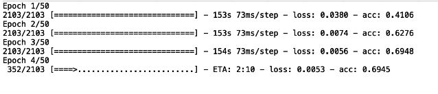
A word of caution
You might see the accuracy going up and think it’s working. But you have to understand that the training image and the label image are almost similar in the first place. So a high accuracy is misleading here. Following the trend, the loss will obviously also be going down like cream but here too, since the images are similar (one blurred, one sharp but of the same picture essentially), the loss will be small to begin with.
After the model has been trained and saved, we can use it for predictions.
Instead of using every image in the test set, we can just test it on one random image from the training set and see how the model is performing.
Because if it does not perform well on images it has seen (training set), it will surely not perform well on the image it has never seen (test set).
This can be done by:
from keras.models import load_model

unblur = load_model(‘/Users/bhargavdesai/Desktop/normal_model.h5’) //path to the saved model
unblur.summary()//print out the summary of the model
test = cv2.imread(‘/Users/bhargavdesai/Downloads/GOPRO_Large/train/GOPR0374_11_00/blur/000002.png’,-1) //path to a random blurred image from train
test_resized = cv2.resize(test,(128,72))
test_scaled = test_resized/255.0 //convert to [0,255] range
test_reshaped = np.reshape(test_scaled, (1,72,128,3))
pred = (unblur.predict(test_reshaped))*255.0
sharp = pred.astype(‘int32’)
sharp = np.reshape(sharp,(72,128,3))
cv2.imwrite(‘sharpened.png’,sharp)
This will write the supposed-to-be sharpened image to the working directory.
Let’s see what we have got:

???????????????
Ummmmm.
Excuse me Neural Network, I’m sorry but I don’t that’s what we had in mind.
This is what the output should actually be resembling:

But the image produced is not sharpened at all.
In fact, it is a blurred image resembling the blurred image more than it resembles the sharpened image!
Well, okay. No problem. Let us change the model structure to include more layers and more epochs. If a simple model couldn’t do the trick, surely a sufficiently complex one would do the trick:
model = Sequential()

#add model layers
model.add(Conv2D(64, (3,3), activation=’relu’, padding=‘same’, input_shape=(128,72,3)))
model.add(Conv2D(64, (3,3), activation=’relu’, padding = ‘same’))
model.add(Conv2D(32, (3,3), activation=’relu’, padding = ‘same’))
model.add(Conv2D(32, (3,3), activation=’relu’, padding = ‘same’))
model.add(Conv2D(16, (3,3), activation=’relu’, padding = ‘same’))
model.add(Conv2D(16, (3,3), activation=’relu’, padding = ‘same’))
model.add(Conv2D(3, (3,3), activation=’relu’, padding = ‘same’))

model.compile(optimizer=‘adam’, loss=’mean_squared_error’, metrics=[‘accuracy’])
model.summary()
model.fit(x=X_train, y=Y_train, epochs = 128, batch_size = 32)
model.save(‘complicated_model.h5’)
After the model is saved, we can rerun the steps to test an image by a new model following the code given above and we will notice almost the exact same result. Take a look:

You can increase the complexity even further. The result will not change. The image will not sharpen. It will resemble the blurred image.
In fact, we have tried increasing the size of the image from (128,72,3) to the maximum and various sizes in between.
You can give it a try too if your machine allows it or use Google Colab, you will get the exact same result.
So what do we do now? Is this problem unsolvable?
Well, it’s taken a while, almost too long if truth be told, but we finally arrive at the usefulness of the Functional API of Keras.
Turns out, there are two ways you can create models in Keras.
1. Sequential
2. Functional
The sequential way is what we have been doing all the way until this blog in the Keras series.
As the word suggests you can just sequentially add layers to your network which seems good enough until you come to face with problems like this one.
The functional way allows you to do much more.
First things first, the import:
from keras.models import Model
from keras.layers import Input, Conv2D, Concatenate
Now building the model:
input_img = Input(shape=(72, 128, 3)) //define shape of input (mandatory)

c1 = Conv2D(32, (9, 9), padding="same", activation="relu")(input_img)
c2 = Conv2D(32, (5, 5), padding="same", activation="relu")(c1)
m= Concatenate(axis=-1)([c1, c2])
c3 = Conv2D(32, (5, 5), padding="same", activation="relu")(m)
c4 = Conv2D(32, (5, 5), padding="same", activation="relu")(c3)
c5 = Conv2D(3, (5, 5), padding="same")(c4)
Three things to notice:
- We don’t use ‘model.add()’ anymore. Instead, we define a layer, for example c1 = Conv2D(32, (9, 9)….. activation=“relu”) and then we just ‘float’ other layers through it. Like, c1 = Conv2D(32, (9, 9)….. activation=“relu”) (input_img).
- The implication of this is that we can mix and match layers, ‘float’ whichever layer we want through which layer. There is no need for an order here. We can even share layers, merge layers, or pass the same input through multiple layers! Functional API allows for immense flexibility, creativity, and space for the AI developer!
- As an example from the model defined above, consider the line, m= Concatenate(axis=-1)([c1, c2]). Here, we have merged or concatenated two layers to create a new layer!
This architecture is actually the DBSRCNN architecture proposed in the paper ‘Image Deblurring And Super-Resolution Using Deep Convolutional Neural Networks’, by F. Albluwi, V. Krylov and R. Dahyot (http://mlsp2018.conwiz.dk/home.htm).
 The basic idea is to extract rudimentary features from the first layer, enhanced features from the second layer, and use the knowledge from BOTH of those layers to make the decision about the output as opposed to only the previous layer features that we have been using in our Sequential model. If you were to train this network, the output you would get would be as follows:


(The expected sharpened image (below) is again shown here for side-by-side comparison)
Which is a lot better with a lot less model complexity than our previous model. Although not perfect, this model works better than the models we created and thought would work with the Sequential API.
Also Read: Dive deep into the basics of Artificial Neural Networks
This is creativity.
This is why we need the Functional API. To allow us the creative space to think beyond the conventional. For example, in this problem, a creative solution was found by using rudimentary and enhanced features from both layers into constructing the sharpened image.
To conclude then, we would like to run over a couple of handy tips in the Functional API to make your experience with it better:
1. Visualizing: The thing about Functional API and all its flexibility is that models tend to get plenty complicated. So to visualize the model architecture, Keras has an inbuilt function, plot_model(). Here is how you use it:
from keras.utils import plot_model
plot_model(model, to_file=‘model.png’)
The plot of the model we created previously, looks as follows:

2. Building Multiple Input Models: Another important use of Functional API is the ability to create submodels that have the same input, but different model architectures so that different submodels can pick up different features from a common input and then at the output the layers are merged using Concatenate() to give a more robust and discerning output.
An example of such a model is given below:

We noticed that even with the DBSRCNN architecture the results weren’t optimum.
We encourage you to try a variation of the model architecture shown above and see if it leads to a better solution?
Meanwhile, you can also check out the “The Deep Learning Masterclass: Classify Images with Keras” tutorial to understand it more practically. The course comes with 6 hours of video that covers 7 important sections. Taught by a subject expert, this course includes topics like Intro to Classes and Objects, If Statements, Intro to Convolutions, Exploring CIFAR10 Dataset, Building the Model and much more.
So, this was it. Leave us comments below about your results and also if you had any doubts following this blog!
Until next time, you can read more by clicking on the links below.
More From The Keras Series:
- Deep Neural Networks with Keras
- Convolutional Neural Networks with Keras
- Recurrent Neural Networks and LSTMs with Keras
- Functional API of Keras


