

Neural Networks
In the previous post, we scratched at the basics of Deep Learning where we discussed Deep Neural Networks with Keras. As a code along with the example, we looked at the MNIST Handwritten Digits Dataset:
You can check out the “The Deep Learning Masterclass: Classify Images with Keras” tutorial to understand it more practically. The course comes with 6 hours of video that covers 7 important sections. Taught by a subject expert, this course includes topics like Intro to Classes and Objects, If Statements, Intro to Convolutions, Exploring CIFAR10 Dataset, Building the Model, and much more.
And after training it on our very own designed, developed and written from scratch Deep Neural Network, we were able to classify each digit correctly with 97.7% accuracy.
If you’ve missed that article, we suggest you head right over to it so that everything in this blog feels seamless.
Whether you are new to AI or been around a while, you’d know the invisible standard protocol:
“If there be an Image, then there shall be a Convolutional Neural Network.”
Read More: Convolutional Neural Networks for Image Processing
But why is that?
You see, in all the engineering and practical science, there is, we can easily single out our obsession with one single thing: efficiency.
And as mentioned in our last discussion, we classified MNIST Handwritten image dataset using a Deep Neural Network, that too with a staggering accuracy of 97.7%.
Now if a tool as effective as a Deep Neural Network already exists, why would you need another at all?
Having two different tools to solve the same task? Isn’t that redundancy, the exact opposite of efficiency?
That’s the quandary. The dilemma.
As it turns out, we will learn two important things from the discussion that ensues:
i. A Deep Neural Network or DNN is wastefully inefficient for image classification tasks.
ii. A Convolutional Neural Network or CNN provides significantly improved efficiency for image classification tasks, especially large tasks.
But let’s take it one step at a time.
At Eduonix, we encourage you to question the rationality of everything.
So it is fitting then, that we start our discussion precisely by unraveling this dilemma first.
We reckon from our brief discussion of the MNIST Handwritten Dataset in the previous article that each image was 28 x 28 x 1 grayscale.
Consequently, we had 784 (28 x 28 x 1) neurons in our input layer handling of which was a piece of cake for any modern processor. The problem is, often most images have way more pixels than that, and even more often they, not grayscale images. To see why this is a problem, the image if each of our handwritten image digit in the MNIST dataset was in 4K Ultra HD. Each image would then be 4096 x 2160 x 3 so basically, we would have had to have 26,542,080 (4096 x 2160 x 3) in the input layer itself, forget the neurons in the hidden layers ahead.
Depending on the use case, we might have thousands or even hundred of thousands of high-quality images which leads to insurmountable numbers. You don’t even want to imagine the load on the processor for a 4K video which may have as many as 60 frames per second. These neuron numbers and the accompanying calculations are not really manageable except by highly sophisticated processors or powerful graphics cards or distributed cluster systems. It is inherently obvious that Deep Neural Networks are neither scalable nor efficient for image classification.
That’s the first part of the story done.
Now to understand the second, we need a quick intuitive dive into the concept of convolution from image processing theory. A fancy jargon really, but way simpler than it sounds. It’s basically just receptive arithmetic. Multiplications and additions.
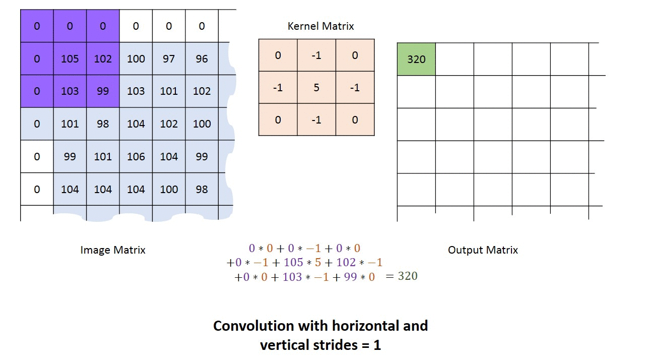
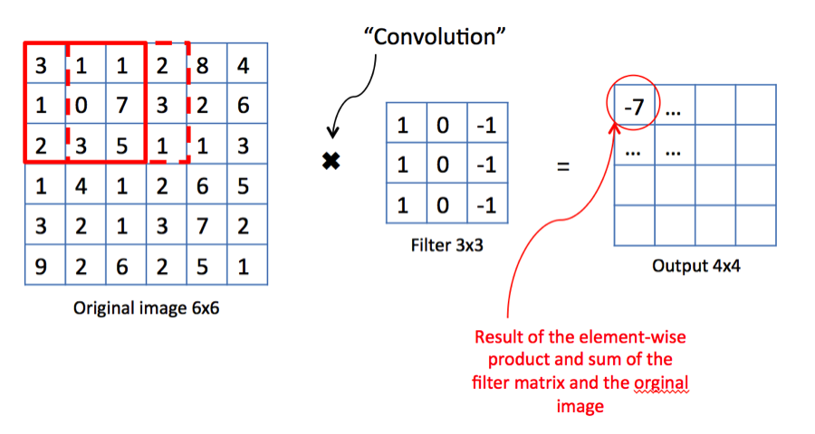
Let’s take a look. Consider the example above.
We have an image, and two alien terms: Kernel Matrix or Filter as it is referred to in image processing theory, and Output Matrix.
Both terms need some explanation but we’ll come to it later.
For now, let us understand the concept of convolution.
We start in the upper lefthand corner by placing the lefthand corner of filter on the underlying image and taking a dot product as shown in the graphic above. We then move the filter across the image step by step until it reaches the upper righthand corner. The size of the step is known as stride. Stride is a hyperparameter because we can move the filter to the right one column at a time, or we can choose to take larger steps. At each step, we take another dot product, and we place the results of that dot product in a third matrix, the output matrix or the activation map, the first alien term.
This is shown in the preceding graphic along with the calculations involved.
Although we have shown only one channel for illustration purposes, the filter actually applies to each channel (RGB) of our image.
Right. Back to the remaining alien term then.
Kernel Matrix:
This is the key that makes Convolutional Neural Networks so efficient. The job of the kernel matrix or filter is to find patterns in the image pixels in the form of features that can then be used for classification. What do we mean by ‘features’ and how can a mere 3×3 matrix be used to generate them? As we say, the best way to learn is by example.
Consider that we want to make a simple system that can classify the English alphabet. Let us use a 3×3 matrix as defined below. On convolving this with an image of letters E and A, we get the following result:
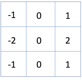
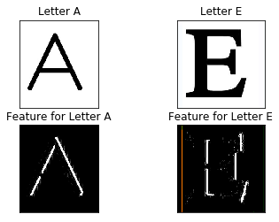
Intuitively, we can manually configure the system to classify letter A on basis of diagonal lines and letter E on the basis of vertical lines which are the features.
Right away we notice that in the previous case, we have defined the filter manually based on our knowledge.
But what if the system were able to learn this filter all by itself?
This is the fundamental concept of a Convolutional Neural Network.
It is the self-learning of such adequate classification filters, which is the goal of a Convolutional Neural Network.
Implementation using Keras
We now come to the final part of this blog, which is the implementation of a CovNet using Keras. The reasons for using Keras have been discussed in the previous article.
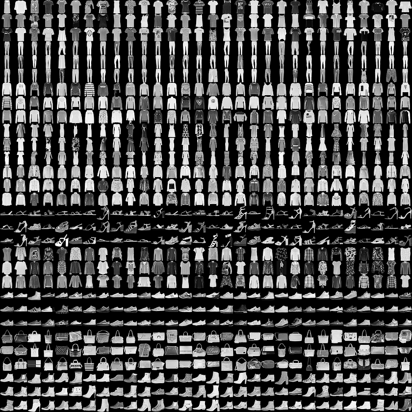
Since we can pride ourself for coming to the next level in AI computer vision algorithms, the dataset we will use is the Fashion MNIST because it is intended as a level up to the classic MNIST dataset, which we described as the “Hello, World” of machine learning programs that we used for Deep Neural Network in the previous article.
About the Dataset
Just as the MNIST dataset contained images of handwritten digits, and Fashion MNIST contains, in an identical format, articles of clothing.
We will use 60,000 images to train the network and 10,000 images to evaluate how accurately the network learned to classify images.
Step 1: Accessing the Dataset
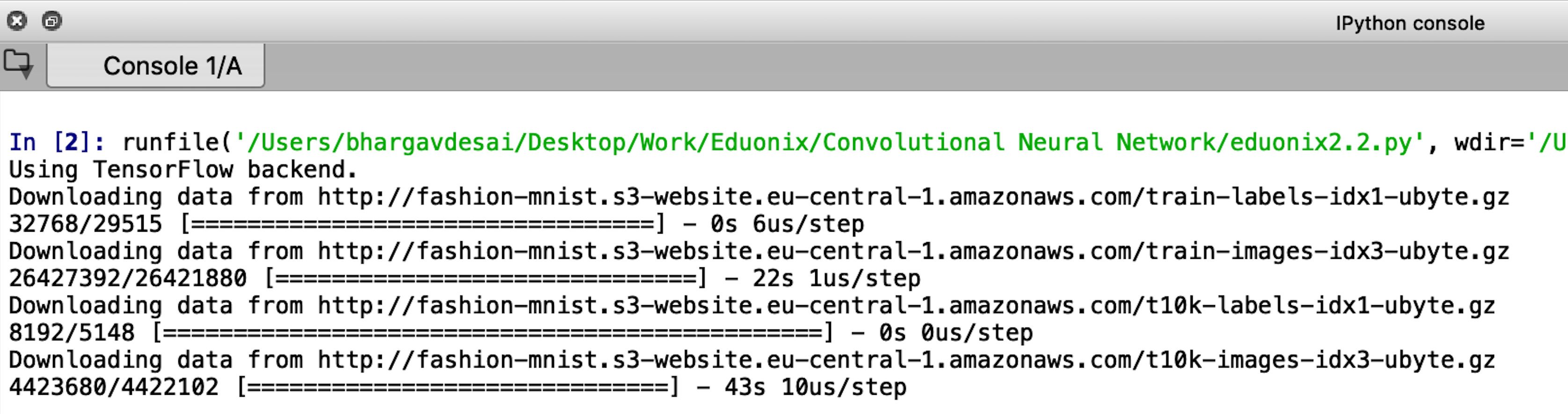
We can access the Fashion MNIST directly from Keras, just import the required libraries and then load the data:
import numpy as np
import tensorflow as tf
import keras
from keras.models import Model
from keras.models import Sequential, load_model
from keras.layers import Dense, Conv2D, Dropout, Flatten, MaxPooling2D
from keras.utils import np_utils

fashion_mnist = keras.datasets.fashion_mnist
(train_images, train_labels), (test_images, test_labels) = fashion_mnist.load_data()
Step 2: Visualising the Dataset and its Properties
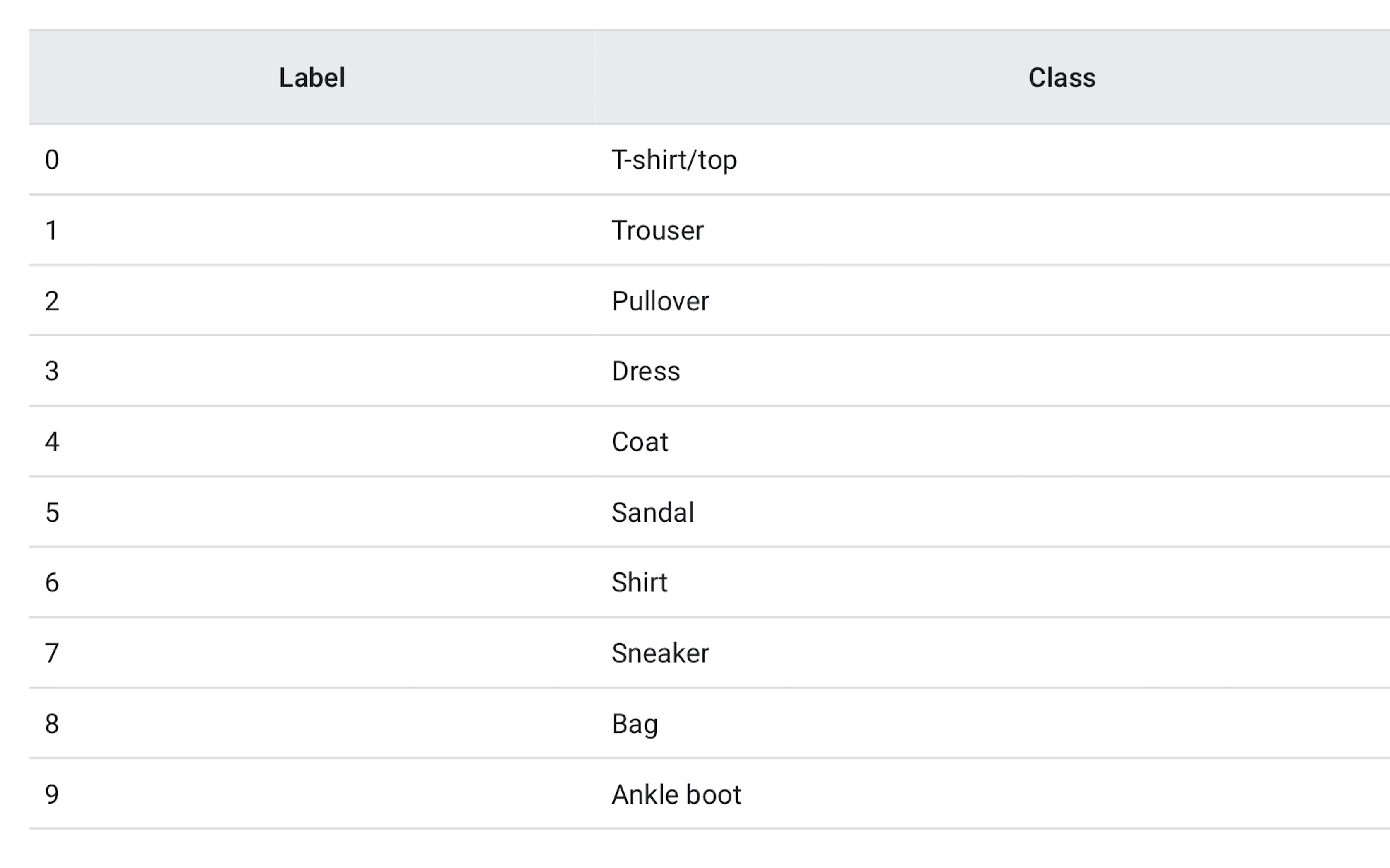
The train_images and train_labels arrays together are the training set which we will use to train the network and the test_images and test_labels arrays are on which we will evaluate the performance of our model. The labels and their classes are given as follows:
The shape of the training and test sets can be verified by:
train_images.shape
Out[3]: (60000, 28, 28)

test_images.shape
Out[4]: (10000, 28, 28)
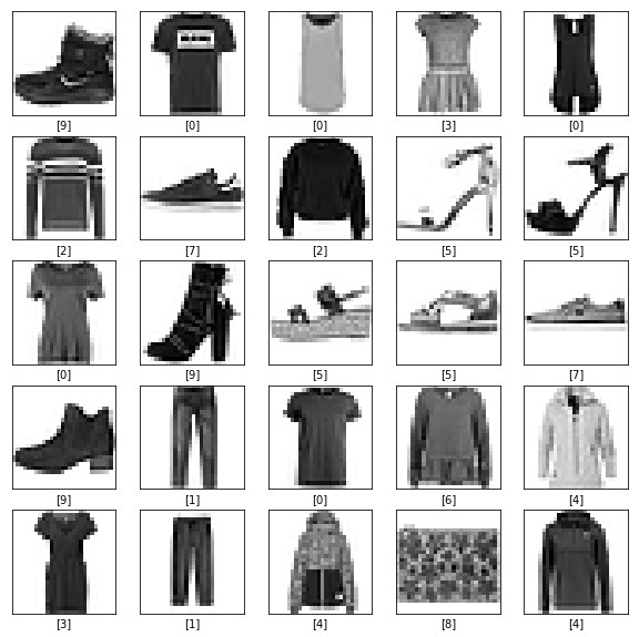
It is always better to visualize data for a quick sanity check. Let’s do that. We will plot the first 25 images with their class labels. The code for this is pretty straightforward.
import matlplotli.plyplot as plt
plt.figure()
for i in range(25):
plt.subplot(5,5,i+1)
plt.xticks([])
plt.yticks([])
plt.grid(False)
plt.imshow(train_images[i], cmap=plt.cm.binary)
plt.xlabel([train_labels[i]])
plt.show()
We encourage you to play around with the plt.xticks([]), plt.yticks([]), plt.grid(False) commands and see how the output changes.
Step 3: Building the Model
A model is nothing but a stack of layers. Focus your attention on the libraries that we imported at the very beginning. Specifically the line:
from keras.layers import Dense, Conv2D, Dropout, Flatten, MaxPooling2D
Let’s go over these layers one by one quickly before we build our final model.
i. Dense: A Dense layer is just a bunch of neurons connected to every other neuron. Basically, our conventional layer in a Deep Neural Network.
ii. Conv2D: This is the distinguishing layer of a CovNet. This is a layer that consists of a set of “filters” which take a subset of the input data at a time, but are applied across the full input, by sweeping over the input as we discuss above. The operations performed by this layer are linear multiplications of the manner that we learned about prior. Keras allows us to define the number of filters along with their size and the stride.
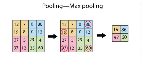
iii. MaxPooling2D: This layer simply replaces each patch in the input with a single output, which is the maximum (can also be average) of the input patch. This is best understood with a diagram:
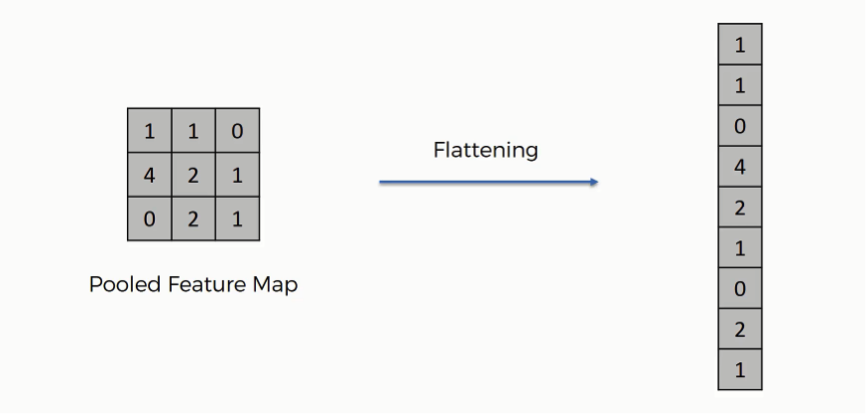
iv. Flatten: This layer just performs an ‘unroll’ operation on an activation map or output matrix so that we can pass it to a Dense layer. Again, let us understand this with an example:
In addition to the layers we have defined above, there is one more layer that is important called the Batch Normalisation Layer which normalizes the activations of each layer, consequently speeding up training.
Finally, our model. If you’ve read the previous blog in this Keras series, you would know that we always start defining our Keras model with the following line of code:
model = Sequential()
This creates a ‘Keras Model’ object, details of which you do not really have to worry about now.
We can now starting building our model by simply ‘adding’ layers to the Model object by model.add(…)
model.add(Conv2D(64, (3, 3), padding=“same”, activation=’relu’, input_shape=(28,28,1)))
model.add(Conv2D(32, (3, 3), padding="same", activation=’relu’))
model.add(MaxPooling2D(pool_size=(2, 2)))
model.add(Conv2D(32, (3, 3), padding="same", activation=’relu’))
model.add(Conv2D(16, (3, 3), padding="same"))
model.add(MaxPooling2D(pool_size=(2, 2)))
model.add(Conv2D(16, (3, 3), padding="same"))
model.add(Conv2D(8, (3, 3), padding="same"))
model.add(MaxPooling2D(pool_size=(2, 2)))
model.add(Flatten())
model.add(Dense(128), activation = ‘relu’)
model.add(Dense(10), activation = ‘softmax’)
model.summary()
Note that the number of neurons in the last dense layer will always be equal to the number of classes we have, which in our case is 10.
Let us go over one of the code lines so that the meaning of this entire model building segment is intuitively clear.
We have mentioned previously that we can define the number of filters as well as the stride of a convolution layer in Keras.
model.add(Conv2D(64, (3, 3), padding=“same”, activation=’relu’, input_shape=(28,28,)))
Here, the first parameter inside the inner parenthesis, 64, defines the number of filters. The next parenthesis (3,3) defines the filter size. The parameter, padding=“same”, requires a bit of additional explanation.
We know from our knowledge of convolution that normally the filter moves covers the entire area in strides from one edge of the image to the other edge.
But there’s a problem here.
When moving the filter this way we see that the pixels on the edges are “touched” less by the filter than the pixels within the image. That means we are throwing away some information related to those positions. Furthermore, the output image is shrinking on every convolution, which could be intentional, but if the input image is small, we quickly shrink it too fast which may result in poor feature extraction and hence poor image classification accuracy.
A solution is the use of “padding”. Before we apply a convolution, we pad the image with zeros all around its border to allow the filter to slide on top and maintain the output size equal to the input. The result of padding in the previous example will be:
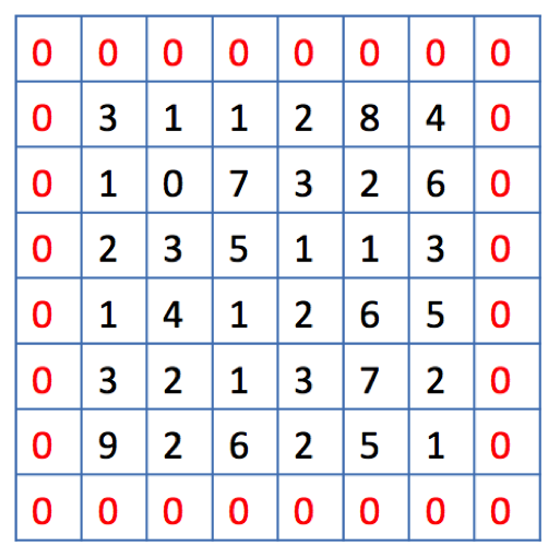
This is what is meant by the padding=“same” parameter.
The input shape is self-explanatory since the size of our images is 28 x 28.
Step 4: Compiling and Training the Model
Before moving on to compile our model, we will normalize our images between 0 and 1 to avoiding vanishing and exploding gradients during network training to increase stability.
We will also one-hot vectorize our training and test labels. The code for this is given below and the reason for these processes are described in greater detail in the previous blog of this series:
train_images = train_images/255.0
test_images = test_images/255.0
train_images = train_images.reshape(60000,28,28,1)
test_images = test_images.reshape(10000,28,28,1)
train_labels = np_utils.to_categorical(train_labels, 10)
test_labels = np_utils.to_categorical(test_labels, 10)
We need to reshape the train_images and test_images the way shown otherwise, Keras will throw your dimensionality errors.
Compiling and training the model in Keras is done in two lines:

model.compile(optimizer=’adam’,
              loss=’categorical_crossentropy’,
              metrics=[‘accuracy’])

model.fit(train_images, train_labels, batch_size=32, epochs=7)

model.save(‘simple_cnn_with_keras.h5’)
del model
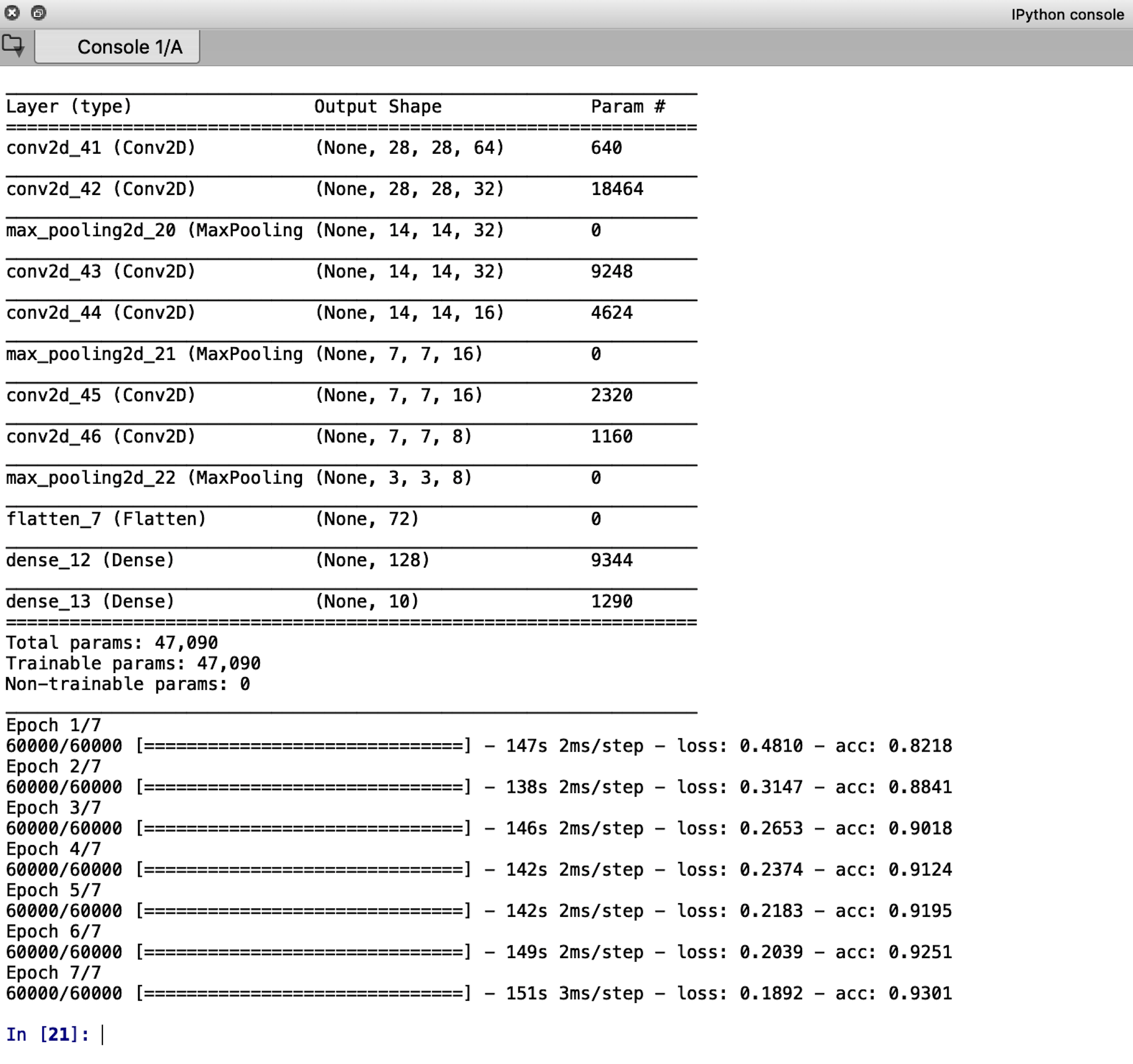
The output screen should look something like this:
Step 5: Testing the Model
We conclude this blog on Convolutional Neural Networks by testing the model we have trained:
cnn_model = load_model(‘simple_cnn_with_keras.h5’)
accuracy_loss = cnn_model.evaluate(test_images, test_labels, verbose=2)
print(“Test Loss”, accuracy_loss[0])
print(“Test Accuracy”, accuracy_loss[1])
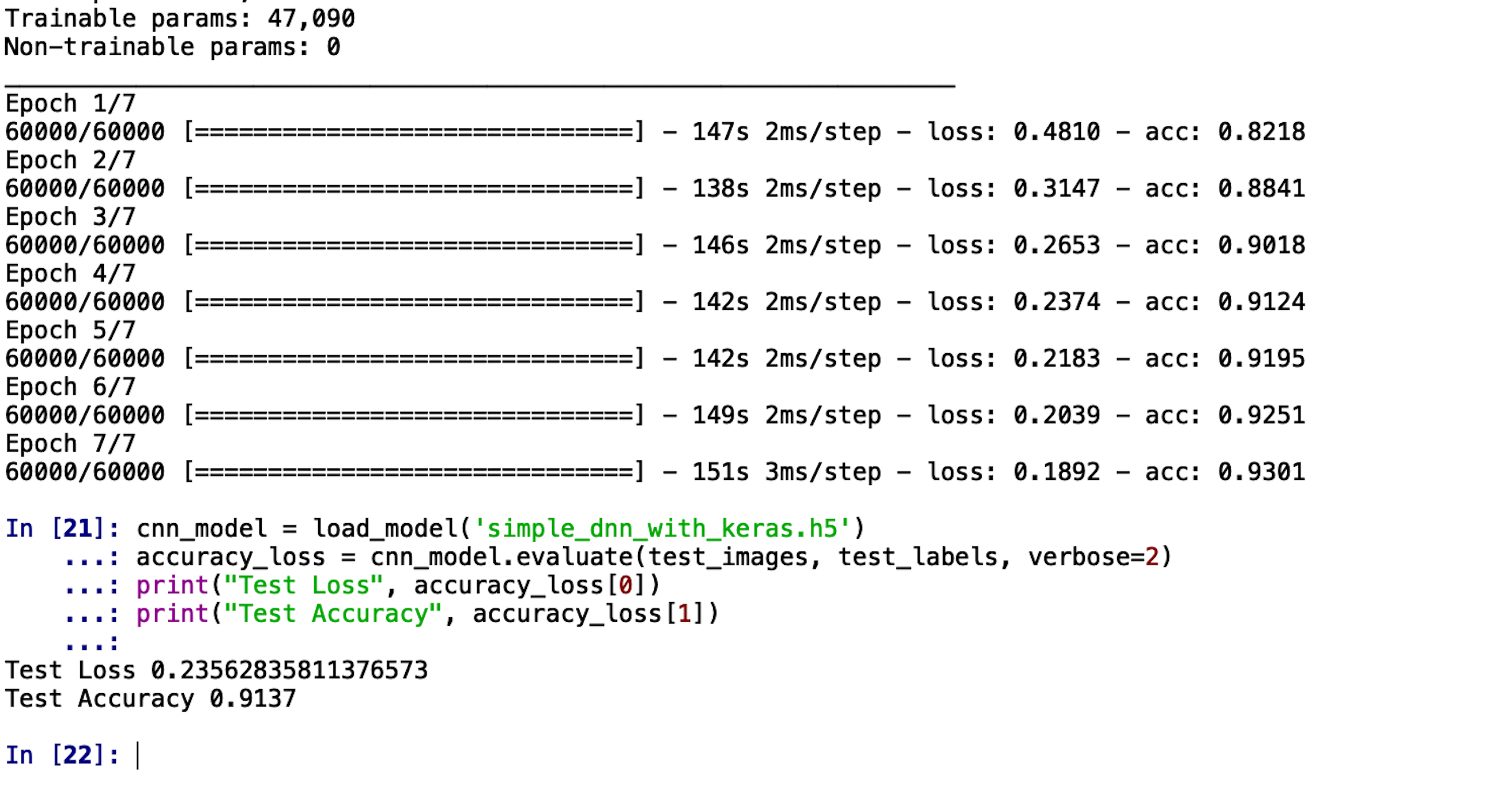
The accuracy we get on unseen images is 91.37%. This means out of the 10,000 images, we got classified 9,137 images correctly! Pretty neat, we’d say!
As a parting challenge, we’d like you to work on the same Dataset and see if you can match this accuracy by a Deep Neural Network discussed in the previous article!
Hit the comment section below with your results!
Let the battle of accuracies begin!
More From The Keras Series:
- Deep Neural Networks with Keras
- Recurrent Neural Networks and LSTMs with Keras
- Functional API of Keras