
Keras
Artificial Intelligence in 2021, is a lot of things.
But I think we all can pretty much agree, hands down, that it’s pretty much Neural Networks, for which the buzz has been about.
I mean, nobody is to blame really because indeed, ‘Neural Networks’ does sound very exotic in the first place.
The question, however, is, are they just that? An exotic-sounding name? Or do they bring something more to the table in the way that they operate and whether they justify the surrounding hype at all?
With the help of this code along with the tutorial blog, these are precisely the questions that we hope we’ll have helped you unravel the answers to, along with making you feel at home about coding up your Neural Networks on your own computer, of course.
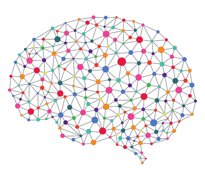
A quick revision before we begin, Neural Networks are computational systems modeled after, well, the human brain, less because of merit and more because of a lack of any other animal brain to model it after. After all, arguably, the notion of higher intelligence and its display outside of the Homosapiens is largely absent.
Don’t believe us? Take a look at the biological model of a neuron (billions of which you have in your head) and one unit of your own Artificial Neural Network which you’ll be coding up in a while:
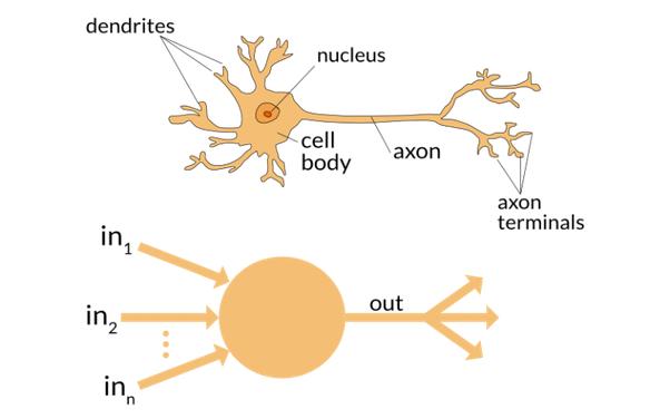
A little crude perhaps, but it is indeed easy to notice the similarities between the two.
Wait a minute. But didn’t we just mentioned that you have billions of these in your head? Well, here’s the catch, we cannot have a billion of these coded on your computer because of the computational memory and processing power constraints, but we can, however, definitely have more than just one.
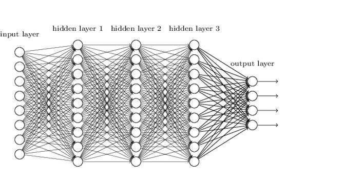
This takes us to the concept of a Deep Neural Network which is really just a fancy name for many of those artificial neurons connected to each other.
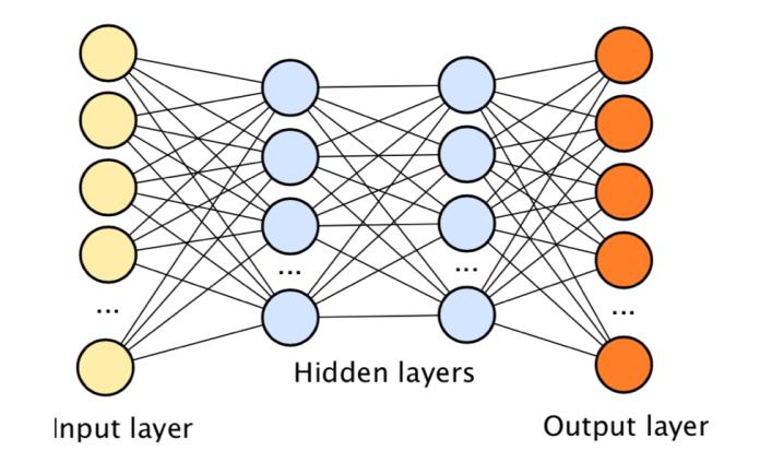
Here’s a representation to see what we mean:
Right. Some terminologies to get out of the way then.
Let us understand these with an example. Say you are trying to build a car detector.
i. Layer: A layer is nothing but a bunch of artificial neurons. You are in control of how many neurons or units you define for a particular layer, of course.
ii. Input Layer: This is where you ‘feed the data in’ to your DNN. In our example, it would be an image that has a car!
iii. Hidden Layer: These are your ‘feature extractors’. Let us consider how your brain would try to spot a car in the given image. First, your brain looks for wheels, then your brain looks for a shape resembling something like a rectangular box, and if your brain finds these qualities, it says, “Hey! That’s a car”. Now if we were to build a car detector using a DNN, the function of the hidden layers, in simple words, is just to extract these features (wheels, rectangular box) and then look for them in a given image. Don’t worry if this concept is still a little ambiguous, we’ll clear it up in a bit when we start to code.
iv. Output Layer: This is just a collection of artificial neurons that outputs the probability with which the network thinks it’s a car!
So far as good.
Now finally coming to the business. How do we code up DNN?
Well, you see, modeling the human brain, is not so easy after all! It involves some calculus, some algebra, and a whole lot of arithmetic.
Also Read: Introduction to Neural Networks With Scikit-Learn
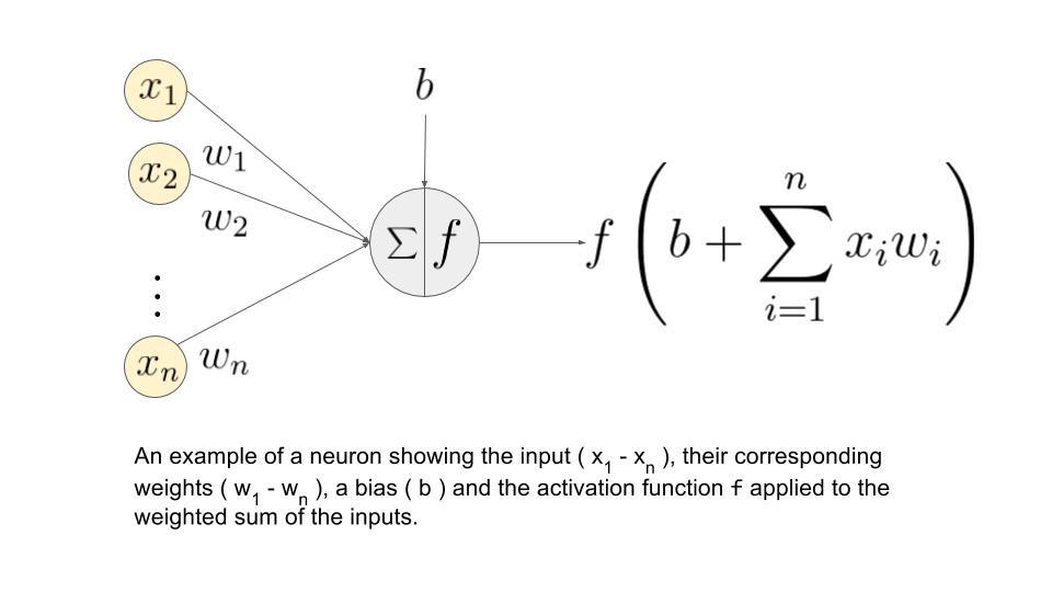
Maybe you are a business owner, looking to learn and incorporate AI and Neural Networks in your business, or perhaps you are a student already familiar with mathematics, endeavoring to do more complicated things with a DNN, you might not always want to spend time writing the basic equations every time because DNN’s can get quite complicated:
Thankfully, there are many high-level implementations that are open source and you can use them directly to code up one in a matter of minutes. One such high-level API is called Keras.
We assume that you have Python on your machine.
If not, here’s where you’ll find the latest version:
We, however, recommend installing Anaconda, especially for
Windows users. It makes life easier, trust us.
Step 1: Install Keras on your machine:
Install Dependencies and Keras:
$ pip install numpy scipy
$ pip install scikit-learn
$ pip install pillow
$ pip install h5py
$ pip install tensorflow
$ pip install keras
Or if you’re using Anaconda, you can simply type in your command prompt or terminal:
conda install -c conda-forge keras
Step 2: Coding up a Deep Neural Network:
We believe in teaching by example. So instead of giving you a bunch of syntaxes you can always find in the Keras documentation all by yourself, let us instead explore Keras by actually taking a dataset, coding up a Deep Neural Network, and reflect on the results.
We learn the basic syntax of any programming language by a
“Hello World” program. It is fitting then, we should begin our learning of Keras with the Hello World of Machine Learning, which the MNIST dataset of Handwriting Digits.
What is the MNIST Dataset?
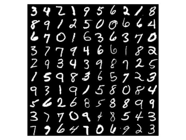
MNIST Dataset is nothing but a database of handwritten digits (0-9).
60,000 training images and 10,000 testing images.
Each handwritten digit in the dataset is a standardized 28×28 gray-scale image which makes it one of the cleanest and compact datasets available as open source in the machine learning world which also contributes to the reason for it being so popular.
Here’s a glance at how the digits look in the actual dataset:
As a matter of fact, Keras allows us to import and download the MNIST dataset directly from its API and that is how we start:
from keras.datasets import mnist
(x_train, y_train), (x_test, y_test) = mnist.load_data()
Using TensorFlow backend.
Downloading data from https://s3.amazonaws.com/img-datasets/mnist.npz
11493376/11490434 [==============================] – 4s 0us/step
You will see your command window display the preceding message once you run those two lines of code.
If you run the line:
x_train.shape
x_test.shape
You’ll get the shapes of the training and test sets.
And as we promised, it is 60,000 and 10,000 images of dimensions 28×28 each.
Out[2]: (60000, 28, 28)
Out[3]: (10000, 28, 28)
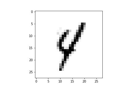
Let us visualize one of these images and see what the image looks like:
import matplotlib.pyplot as plt
image_number= 3457
print(“The label for the image being displayed is:”)
print(y_train[image_number])
plt.imshow(x_train[image_number], cmap=’Greys’)
The output should like the following. You can change the
“image_number” variable to any one of the 60,000 values and you should be able to see the image and its corresponding label which is stored in the (y_train) variable. Visualizing your data is always a good sanity check which can prevent easily avoidable mistakes.
The label for the image being displayed is:
4
Before we come to building our own DNN, there are three considerations that we need to talk a bit about:

I. If we were to take a look at the graphic of a DNN provided earlier in this blog, which we have posted below again for convenience, we notice that the ‘Input Layer’ has just one long line of artificial neurons. Now that’s a hassle because, in our data, we have each image as 28×28.
So we need to ‘unroll’ our 28×28 dimension image, into one long vector of length 28×28 = 786.
This can be done by the reshape function of numpy as shown:
X_train = x_train.reshape(60000, 784)
X_test = x_test.reshape(10000, 784)
II. Since the images are gray-level pixels, each value of an individual pixel can be anywhere from between 0 to 255. The range is thus (Max – Min = 255-0 = 255). If we were to reduce this range from 255 to say between 0 to 1, it would help the neural network learn faster since the dynamic range is much lesser now. This is called Normalisation.
It can easily be done like this:
X_train /= 255
X_test /= 255
III. Thus far, our labels (y_train) and (y_test) variables, hold integer values from 0 to 9. Let’s encode our categories using a technique called one-hot encoding. The result of this will be a vector which will be all zeroes except in the position for the respective category. Thus a ‘6’ will be represented by [0,0,0,0,0,1,0,0,0]. We can do this by writing the code:
Y_train = np_utils.to_categorical(y_train, 10)
Y_test = np_utils.to_categorical(y_test, 10)
We finally concentrate on actually building the model. The model can be built as a Sequential or Functional, but we consider the Sequential API for now. The Functional API will be covered in later blogs when we take on more complicated problems.
We first, define a Sequential model by the following syntax
model = Sequential()
Adding layers to this model is now done simply with the .add() function as demonstrated:
from keras.models import Sequential, load_model
from keras.layers.core import Dense, Activation
from keras.utils import np_utils

model.add(Dense(512, input_shape=(784,)))
model.add(Activation(‘relu’))
model.add(Dense(256))
model.add(Activation(‘relu’))
model.add(Dense(128))
model.add(Activation(‘relu’))
model.add(Dense(10))
model.add(Activation(‘softmax’))
It is intuitively clear that our model architecture has three hidden layers of units 512, 256 and 128 respectively. The first layer is the input layer and the final layer is the output layer with 10 artificial neurons (which is the number of categories that we have, i.e, 0-9)
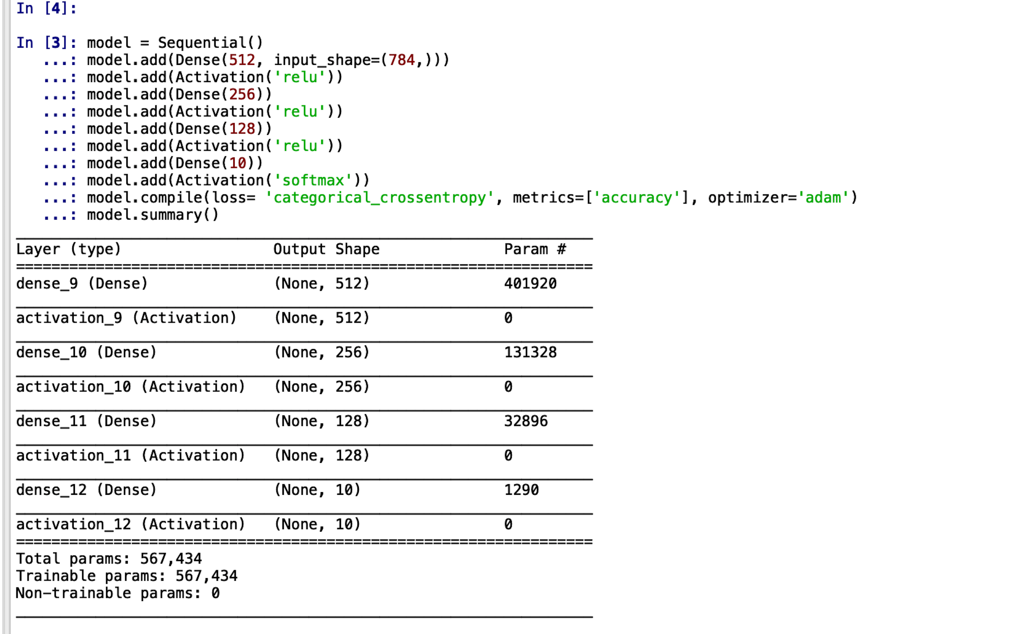
To cross verify this, Keras provides a useful function: model.summary()
The output should look something like this which gives us a good idea of our model architecture.
We now need to compile and train our model. This is the final step.
model.compile(loss=‘categorical_crossentropy’,
metrics=[‘accuracy’],optimizer=’adam’)
We have to specify how many times we want to iterate on the whole training set (epochs) and how many samples we use for one update to the model’s weights (batch size).
Both of these parameters can be tuned to optimize the final accuracy of the model. The optimizations are not covered in this blog.
Model training:
model.fit(X_train, Y_train, batch_size=256, epochs=16, verbose=2, validation_data=(X_test, Y_test))
Saving the model to the working directory and flushing the model from RAM:
model.save(‘simple_dnn_with_keras.h5’)
del model
That is it.
This is all that needs to be done.
You have successfully trained for yourself a Deep Neural Network to recognize handwritten digits with Keras.
But those are just our words.
You need to see for yourself that the classifier actually works.
Also Read: Convolutional Neural Networks for Image Processing
Before we show how to evaluate the model on a test set, just for a sanity check, here is how the output of your code should look like while it’s training.
We should not be very happy just because we see 97-98% accuracy here. A deep enough Neural Network will almost always fit the data.
What is important, is whether the Network has actually learned something or not. That is, we need to see if the Network has just ‘by hearted’ or whether it has actually ‘learned’ something too.
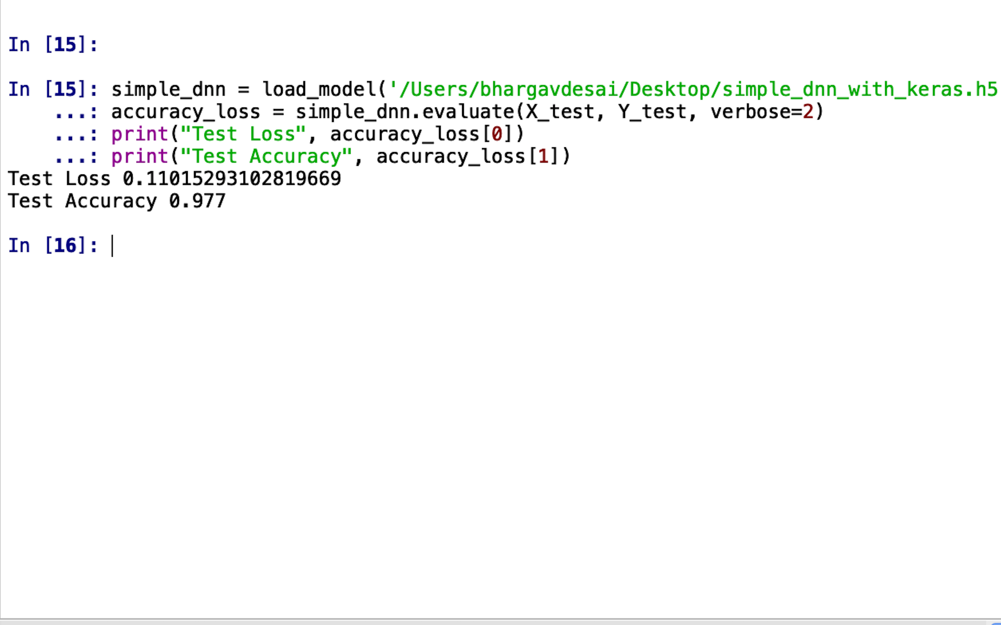
simple_dnn = load_model(‘file_path’). %Your saved model path should be inserted here%
accuracy_loss = simple_dnn.evaluate(X_test, Y_test, verbose=2)
print(“Test Loss”, accuracy_loss[0])
print(“Test Accuracy”, accuracy_loss[1])
Running the above piece of code will give you something like this:
Hey! It looks like our Deep Neural Network did well! 97.7%
accuracy on images it has never seen means that it learned something useful!
Now, to answer the question with which we began our discussion, we would like to reveal an important detail that we didn’t earlier. We could have chosen any dataset available on the internet, why did we choose just this one?
Apart from the generic reasons provided earlier, a more authentic reason for our selection is that the MNIST Dataset is a standard when it comes to image processing algorithms as well.
The image processing algorithms used to solve the exact same problem of categorizing the handwritten digits are vast and very versatile ranging from Adaptive Thresholding to Histogram Modelling all of which, although intuitively simple, require many steps in between input and the classifier.
Whereas a Neural Network abstracts all of those intermediate steps in its hidden layers and consequently, it takes no human involvement whatsoever.
This advantage of abstraction becomes more and more important as we begin to consider even more complicated problems and datasets that would proportionally take even more intermediate processing by normal algorithms.
This is what Neural Networks brings to the table. With problems becoming increasingly complex, instead of manual engineering every algorithm to give a particular result, we give the input to a Neural Network and provide the desired result and the Neural Network figures everything in between.
With this, of course, comes the tradeoff of requiring the large computational capacity to train a Neural Network for more complicated problems, but with Moore’s law well in effect, the processor capacities keep on doubling which has made devices like Alexa and Google Home possible and it is a foregone conclusion that such devices will only continue to be developed going into the future.
If this article has already intrigued you and you want to learn more about Deep Neural networks with Keras, you can try the ‘The Deep Learning Masterclass: Classify Images with Keras’ online tutorial. The course comes with 6 hours of video and covers many imperative topics such as an intro to PyCharm, variable syntax and variable files, classes, and objects, neural networks, compiling and training the model, and much more!
Let us know in the comments below if you found this article informative!
More From The Keras Series:
- Deep Neural Networks with Keras
- Convolutional Neural Networks with Keras
- Recurrent Neural Networks and LSTMs with Keras
- Functional API of Keras