
In the previous blog, we have learned how to create Dynamic Map Using ggmap & RDynamic Map Using ggmap in R. Here, we will focus on creating various types of dynamic maps using ggplot2.
Scatter Plots are similar to line graphs which are usually used for plotting. The scatter plots show how much one variable is related to another. The relationship between variables is called correlation which is usually used in statistical methods.
We will use the same dataset called “Iris” which includes a lot of variation between each variable. This is a famous dataset that gives measurements in centimeters of the variables sepal length and width with petal length and width for 50 flowers from each of the 3 species of iris. The species are nothing but called Iris setosa, versicolor and virginica.
Following steps are involved for creating scatter plots with “ggplot2” package:
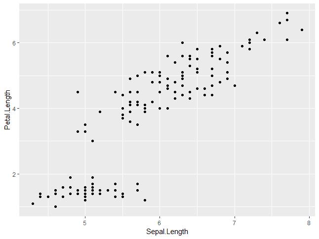
Step 1: For creating a basic scatter plot following command is executed
   # Basic Scatter Plot
> ggplot(iris, aes(Sepal.Length, Petal.Length)) +
+     geom_point()
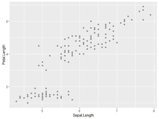
Step 2: We can change the shape of points with a property called shape in geom_point() function.
> # Change the shape of points
> ggplot(iris, aes(Sepal.Length, Petal.Length)) +
+     geom_point(shape=1)
Step 3: We can add color to the points which are added in the required scatter plots.
> ggplot(iris, aes(Sepal.Length, Petal.Length, colour=Species)) +
+     geom_point(shape=1)
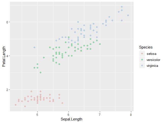
In this example, we have created colors as per species which are mentioned in legends. The three species are uniquely distinguished in the mentioned plot.
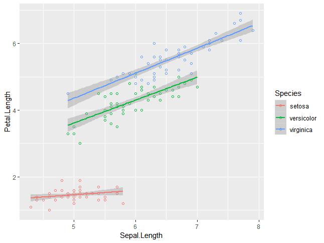
Step 4: Now we will focus on establishing a relationship between the variables.
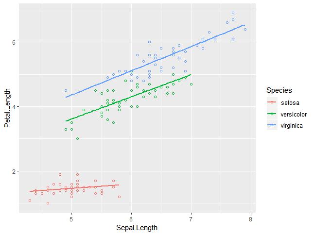
> ggplot(iris, aes(Sepal.Length, Petal.Length, colour=Species)) +
+     geom_point(shape=1) +
+     geom_smooth(method=lm)
geom_smooth function aids the pattern of overlapping and creating the pattern of required variables.
The attribute method “lm” mentions the regression line which needs to be developed.
> # Add a regression line
> ggplot(iris, aes(Sepal.Length, Petal.Length, colour=Species)) +
+     geom_point(shape=1) +
+     geom_smooth(method=lm)
Step 5: We can also add a regression line with no shaded confidence region with the below-mentioned syntax:
># Add a regression line but no shaded confidence region
> ggplot(iris, aes(Sepal.Length, Petal.Length, colour=Species)) +
+     geom_point(shape=1) +
+     geom_smooth(method=lm, se=FALSE)
Shaded regions represent things other than confidence regions.
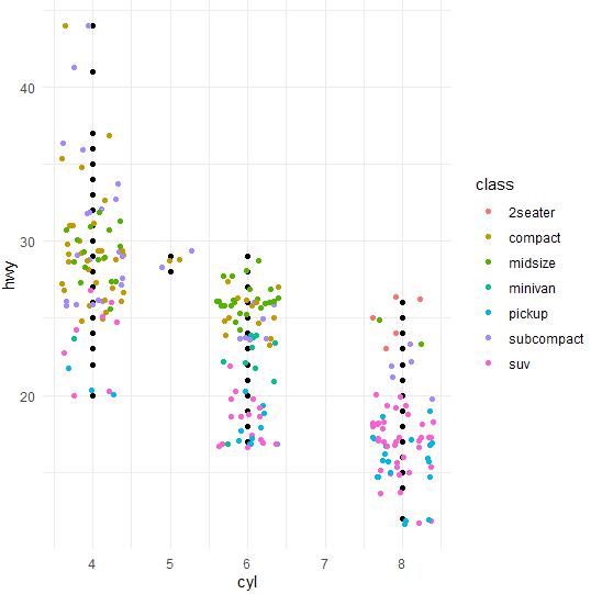
Step 6: Jitter plots include special effects with which scatter plots can be depicted. Jitter is nothing but a random value that is assigned to dots to separate them as mentioned below:
> ggplot(mpg, aes(cyl, hwy)) +
+   geom_point() +
+   geom_jitter(aes(colour = class))
Bar plots represent the categorical data in a rectangular manner. The bars can be plotted vertically and horizontally. The heights or lengths are proportional to the values represented in graphs. The x and y axes of bar plots specify the category which is included in a specific data set.
The histogram is a bar graph that represents the raw data with a clear picture of the distribution of the mentioned data set. In this chapter, we will focus on the creation of bar plots and histograms with help of ggplot2.
Following steps are used to create bar plots and histograms with ggplot2:
Step 1: Let us understand the data set which will be used. Mpg data set contains a subset of the fuel economy data that the EPA makes available on
http://fueleconomy.gov.
It consists of models that had a new release every year between 1999 and 2008. This was used as a proxy for the popularity of the car. The following command is executed to understand the list of attributes that are needed for the data set.
> library(ggplot2)


Attaching package: ggplot2

The following object is masked _by_ .GlobalEnv:

   mpg
Warning messages:
1: package arules was built under R version 3.5.1
2: package tuneR was built under R version 3.5.3
3: package ggplot2 was built under R version 3.5.3
> # Read in dataset
> data(mpg)
> head(mpg)
# A tibble: 6 x 11
 manufacturer model displ  year   cyl trans      drv     cty   hwy fl    class
 <chr>        <chr> <dbl> <int> <int> <chr>      <chr> <int> <int> <chr> <chr>
1 audi         a4      1.8  1999     4 auto(l5)   f        18    29 p     compact
2 audi         a4      1.8  1999     4 manual(m5) f        21    29 p     compact
3 audi         a4      2    2008     4 manual(m6) f        20    31 p     compact
4 audi         a4      2    2008     4 auto(av)   f        21    30 p     compact
5 audi         a4      2.8  1999     6 auto(l5)   f        16    26 p     compact
6 audi         a4      2.8  1999     6 manual(m5) f        18    26 p     compact
>
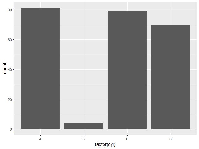
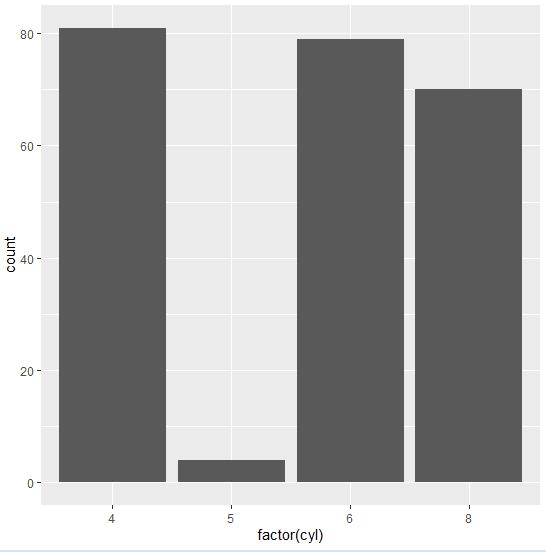
Step 2: The bar count plot can be created with the following command:
> # A bar count plot
> p <- ggplot(mpg, aes(x=factor(cyl)))+
+     geom_bar(stat="count")
> p
geom_bar() is the function that is used for creating bar plots. It takes the attribute of statistical value called count.
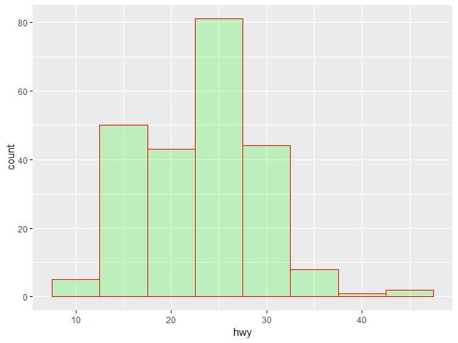
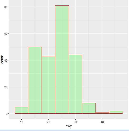
Step 3: The histogram count plot can be created with the below-mentioned plot:
> # A histogram count plot
> ggplot(data=mpg, aes(x=hwy)) +
+     geom_histogram( col="red",
+                     fill="green",
+                     alpha = .2,
+                     binwidth = 5)
geom_histogram() includes all the necessary attributes for creating a histogram. Here, it takes the attribute of hwy with the respective count. The color is taken as per the requirements.
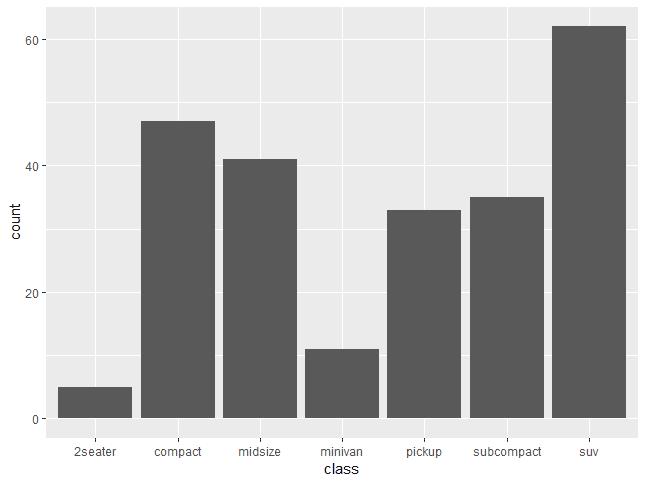
Step 4: The general plots of bar graphs and histograms can be created as below:
> p <- ggplot(mpg, aes(class))
>
> p +  geom_bar()


> p +  geom_bar()
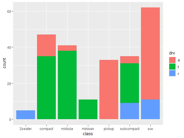
This plot includes all the categories defined in bar graphs with the respective class. This plot is called a stacked graph.
Now, we will focus on the creation of multiple plots which can be further used to create 3-dimensional plots. The list of plots which will be covered include:
- Density Plot
- Box Plot
- Dot Plot
- Violin Plot
We will use the “mpg” dataset as used in previous chapters. This dataset provides fuel economy data from 1999 and 2008 for 38 popular models of cars. The dataset is shipped with a ggplot2 package. It is important to follow the below-mentioned steps to create different types of plots.
> # Load Modules
> library(ggplot2)
>
> # Dataset
> head(mpg)
# A tibble: 6 x 11
  manufacturer model displ  year   cyl trans      drv     cty   hwy fl    class
  <chr>        <chr> <dbl> <int> <int> <chr>      <chr> <int> <int> <chr> <chr>
1 audi         a4      1.8  1999     4 auto(l5)   f        18    29 p     compa~
2 audi         a4      1.8  1999     4 manual(m5) f        21    29 p     compa~
3 audi         a4      2    2008     4 manual(m6) f        20    31 p     compa~
4 audi         a4      2    2008     4 auto(av)   f        21    30 p     compa~
5 audi         a4      2.8  1999     6 auto(l5)   f        16    26 p     compa~
6 audi         a4      2.8  1999     6 manual(m5) f        18    26 p     compa~
Density Plot
A density plot is a graphic representation of the distribution of any numeric variable in the mentioned dataset. It uses a kernel density estimate to show the probability density function of the variable.
“ggplot2” package includes a function called geom_density() to create a density plot.
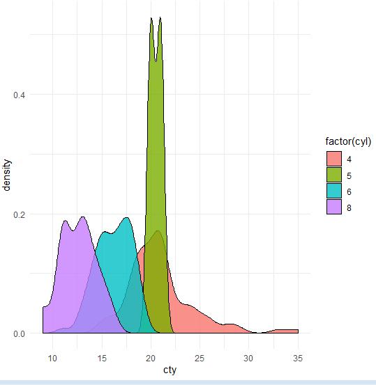
We will execute the following command to create a density plot:
> p <- ggplot(mpg, aes(cty)) +
+   geom_density(aes(fill=factor(cyl)), alpha=0.8)
> p
We can observe various densities from the plot created below:
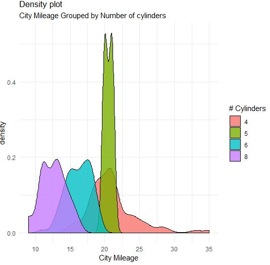
We can create the plot by renaming the x and y axes which maintain better clarity with the inclusion of title and legends with the different color combinations.
> p + labs(title="Density plot",
+        subtitle="City Mileage Grouped by Number of cylinders",
+        caption="Source: mpg",
+        x="City Mileage",
+        fill="# Cylinders")
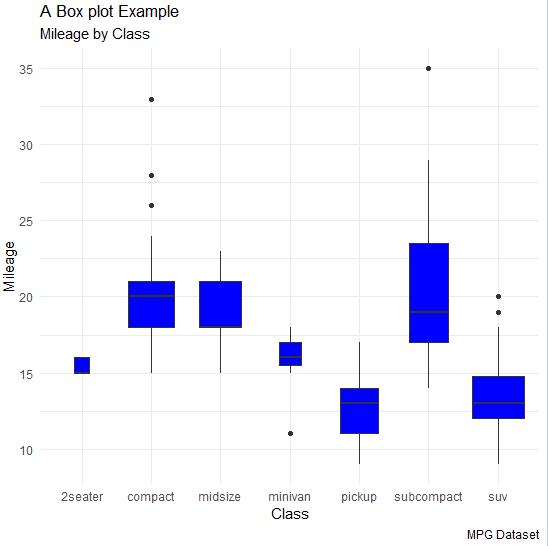
Box Plot
Box plot also called a box and whisker plot represents the five-number summary of data. The five-number summaries include values like minimum, first quartile, median, third quartile and maximum. The vertical line which goes through the middle part of the box plot is considered as “median”.
We can create a box plot using the following command:
> p <- ggplot(mpg, aes(class, cty)) +
+   geom_boxplot(varwidth=T, fill="blue")
> p + labs(title="A Box plot Example",
+        subtitle="Mileage by Class",
+        caption="MPG Dataset",
+        x="Class",
+        y="Mileage")
>p
Here, we are creating a box plot with respect to attributes of class and city.
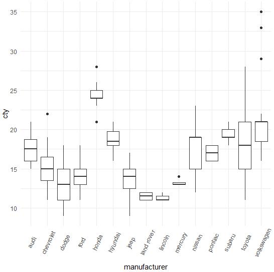
Dot Plot
Dot plots are similar to scatter plots with the only difference of dimension. In this section, we will be adding a dot plot to the existing box plot to understand better pictures and clarity.
The box plot can be created using the following command:
> p <- ggplot(mpg, aes(manufacturer, cty)) +
+   geom_boxplot() +
+   theme(axis.text.x = element_text(angle=65, vjust=0.6))
> p
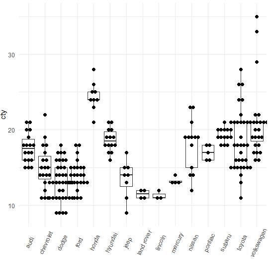
The dot plot is created as mentioned below:
> p  + geom_dotplot(binaxis='y',
+                stackdir='center',
+                dotsize = .5
+                )
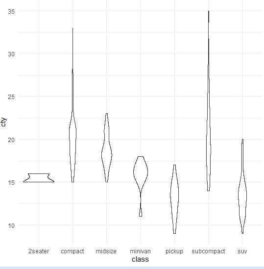
Violin Plot
The Violin plot is also created in a similar manner with only a structure change of violins instead of the box. The output is clearly mentioned below:
> p <- ggplot(mpg, aes(class, cty))
>
> p + geom_violin()
Bubble plots are nothing but bubble charts which is basically a scatter plot with a third numeric variable used for circle size. In this chapter, we will focus on the creation of bar count plot and histogram count plots which are considered as replicas of bubble plots.
Following steps are used to create bubble plots and count charts with mentioned package:
Step 1: Load the respective package and the required dataset to create the bubble plots and count charts.
> # Load ggplot
> library(ggplot2)
>
> # Read in dataset
> data(mpg)
> head(mpg)
# A tibble: 6 x 11
  manufacturer model displ  year   cyl trans      drv     cty   hwy fl    class
  <chr>        <chr> <dbl> <int> <int> <chr>      <chr> <int> <int> <chr> <chr>
1 audi         a4      1.8  1999     4 auto(l5)   f        18    29 p     compa~
2 audi         a4      1.8  1999     4 manual(m5) f        21    29 p     compa~
3 audi         a4      2    2008     4 manual(m6) f        20    31 p     compa~
4 audi         a4      2    2008     4 auto(av)   f        21    30 p     compa~
5 audi         a4      2.8  1999     6 auto(l5)   f        16    26 p     compa~
6 audi         a4      2.8  1999     6 manual(m5) f        18    26 p     compa~
Step 2: The bar count plot can be created using the following command:
> # A bar count plot
> p <- ggplot(mpg, aes(x=factor(cyl)))+
+   geom_bar(stat="count")
> p
Step 3: The histogram count plot can be created using the following command:
> # A histogram count plot
> ggplot(data=mpg, aes(x=hwy)) +
+   geom_histogram( col="red",
+                  fill="green",
+                  alpha = .2,
+                  binwidth = 5)
Step 4: Now let us create the most basic bubble plot with the required attributes of increasing the dimension of points mentioned in a scattered plot.
ggplot(mpg, aes(x=cty, y=hwy, size = pop)) +geom_point(alpha=0.7)
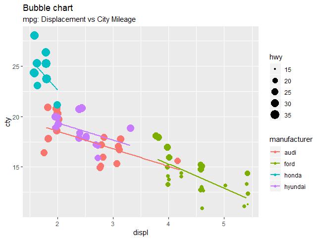
The plot describes the nature of manufacturers which is included in legend format. The values represented include various dimensions of “hwy” attribute.
So, this was all about creating various dynamic maps like different types of scatter plot, jitter plots, bar plot, histogram, density plot, box plot, dot plot, violin plot, bubble plot & others using ggplot2.
In the next section, we will be going to learn about 3D Visualization using different tools of the R programming language.