

As the world battles out the COVID-19 pandemic, our sincere prayers are with the families of the affected. But as the great Benjamin Franklin once said, “Out of adversity, comes opportunity”, & honestly, what better time than now to up our skills and learn something new? Considering this, I have written this article that will help you to build neural networks with PyTorch!
So here we are, marching on from the first blog (PyTorch: The Dark Horse of Deep Learning Frameworks) to the second in this PyTorch series that we’re genuinely excited to bring to our learners! And that’s not all folks! To make sure our students use their quarantined time productively, we’ve released several courses on Eduonix where the only thing we’ll be charging, is dedication! Be sure to check them out!
Since it’s been a while, here is a quick recap of what we covered in the previous blog of this series:
- Why learn PyTorch? We showed several trend graphs for overwhelming growth in the usage of PyTorch in academia, job postings, and the industry making valid cases for learners, practitioners, and hobbyists alike to invest their time in PyTorch.
- We went over some basic syntax such as installation, defining tensors, performing addition, multiplication operations with those tensors, and looked at the NumPy – PyTorch compatibility. We talked about dynamic computation graphs and finally, we highlighted the key differences between NumPy arrays and Torch tensors with proper speed tests where we concluded PyTorch was at least an order of magnitude faster than NumPy.
Read More: Glimpse of PyTorch framework!
While the first blog was aimed at understanding what PyTorch is, what it isn’t and some basic syntax, by the end of this blog we will actually build a full-fledged Neural Network with PyTorch. So let’s look forward to it!
Since most of our learners are familiar with Tensorflow (Keras), throughout this blog we’ll be comparing and contrasting the two libraries so that by the end of this series, the link to Tensorflow is always maintained and there is no ambiguity in whichsoever deep learning library you are tasked with coding in!
Being Keras users for a while now, first up, let’s look at the general “flow” we all think of when someone says “train a model”.
Read More: Implementing Neural Networks with Tensorflow!
The “Flow” we’re used to.
After getting all the data you want to train on in two arrays, X_train and Y_train, it goes something like this:
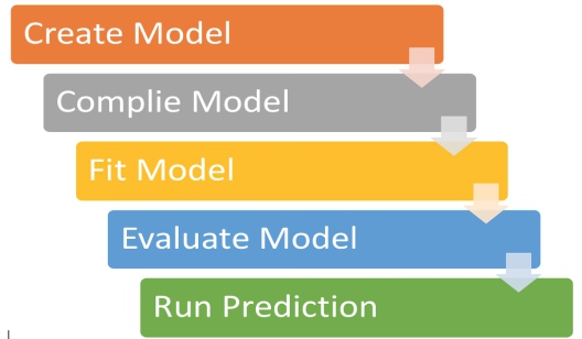
- Define a model using the Sequential or Functional API in Tensorflow (Keras).
- Compile the model using model.complie(), defining your optimizer and loss function.
- Use the model.fit() method to begin training on the compiled model.
- After training, calculate various evaluation metrics like accuracy, loss, etc. and make changes (hyperparameter tuning) if required.
- Use the final model to predict data for the task given in an actual scenario.
We’ll call this the Tensorflow (Keras) model training “Life-Cycle” and is summarised below in Fig. 1 below:
PyTorch on the other hand, does the exact same thing albeit a little differently, offering more flexibility and support than the seemingly “simpler” Keras.
Before we get to it though, you’ll need a brief overview of all the modules you’ll be using while building a Neural Network in PyTorch. Let’s head over to Fig. 2 and check out the modules that we will primarily be needing.
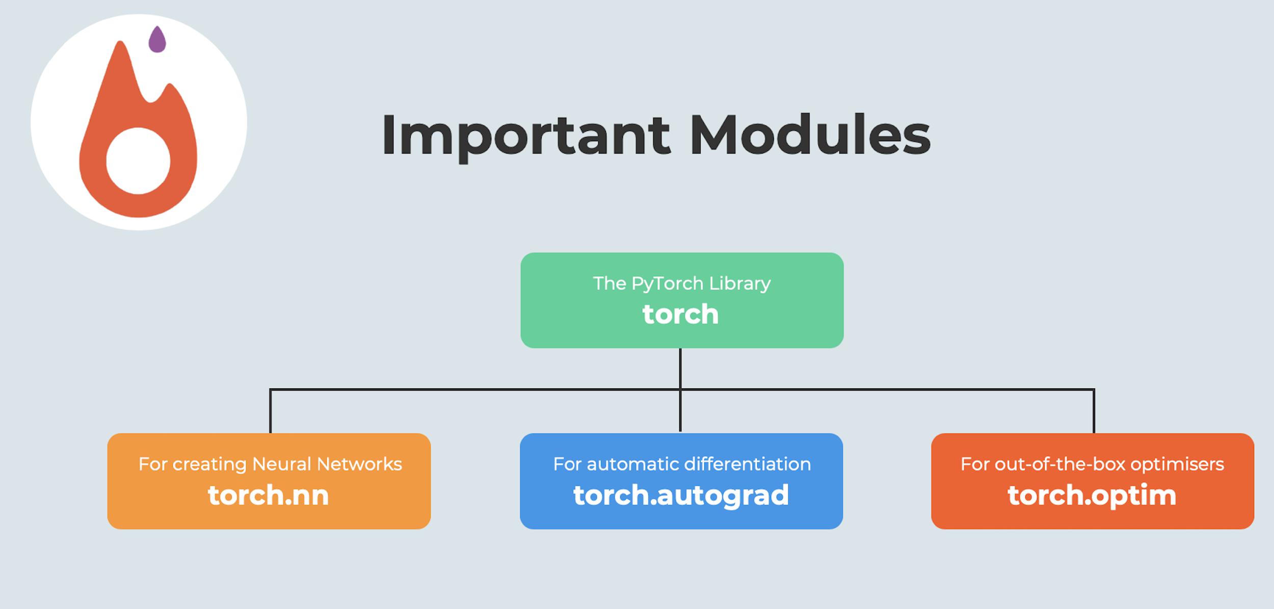
Out of the three modules mentioned in Fig. 2, perhaps the most important is the torch.autograd module. What exactly is this module and why do we need it? Well, you’re about to find out!
Read More: Neural Network- Chronicles of Major Milestones
The Autograd Module.
Autograd is the Automatic Differentiation functionality built into PyTorch. It might seem a little funny since it’s for the first time, TensorFlow, and Keras users are hearing this term. We never needed it while coding networks in Keras did we? The thing is, Automatic Differentiation is a building block of not only PyTorch, but every Deep Learning library out there including TensorFlow. The very reason we love these high-level APIs, which is their ability to abstract away much of the mathematical complexity, is also why we sometimes tend to forget that there’s a ton of calculus happening under the hood. Since nobody really talks about these aspects of Deep Learning, we think now would be a good time to give ourselves a refresher of all the math that’s happening beneath the wrapper functions of any Deep Learning library. (Don’t make that face, we promise it’ll come together by the end of this blog! Stay strong!)
We’ll begin with this. We know that from a computational point of view, training a neural network consists of two phases:
- A forward pass to compute the value of the loss function.
- A backward pass to compute the gradients of the learnable parameters.
The forward pass is pretty straight forward. The output of one layer is the input to the next and so forth. The backward pass is a bit more complicated since it requires us to use the chain rule to compute the gradients of weights w.r.t to the loss function.
A Toy Example.
Nothing quite teaches like an example so let’s step through those two phases of training with the simplest of Neural Networks. We’ll name it the “Back to Basics” network and it looks something like this:
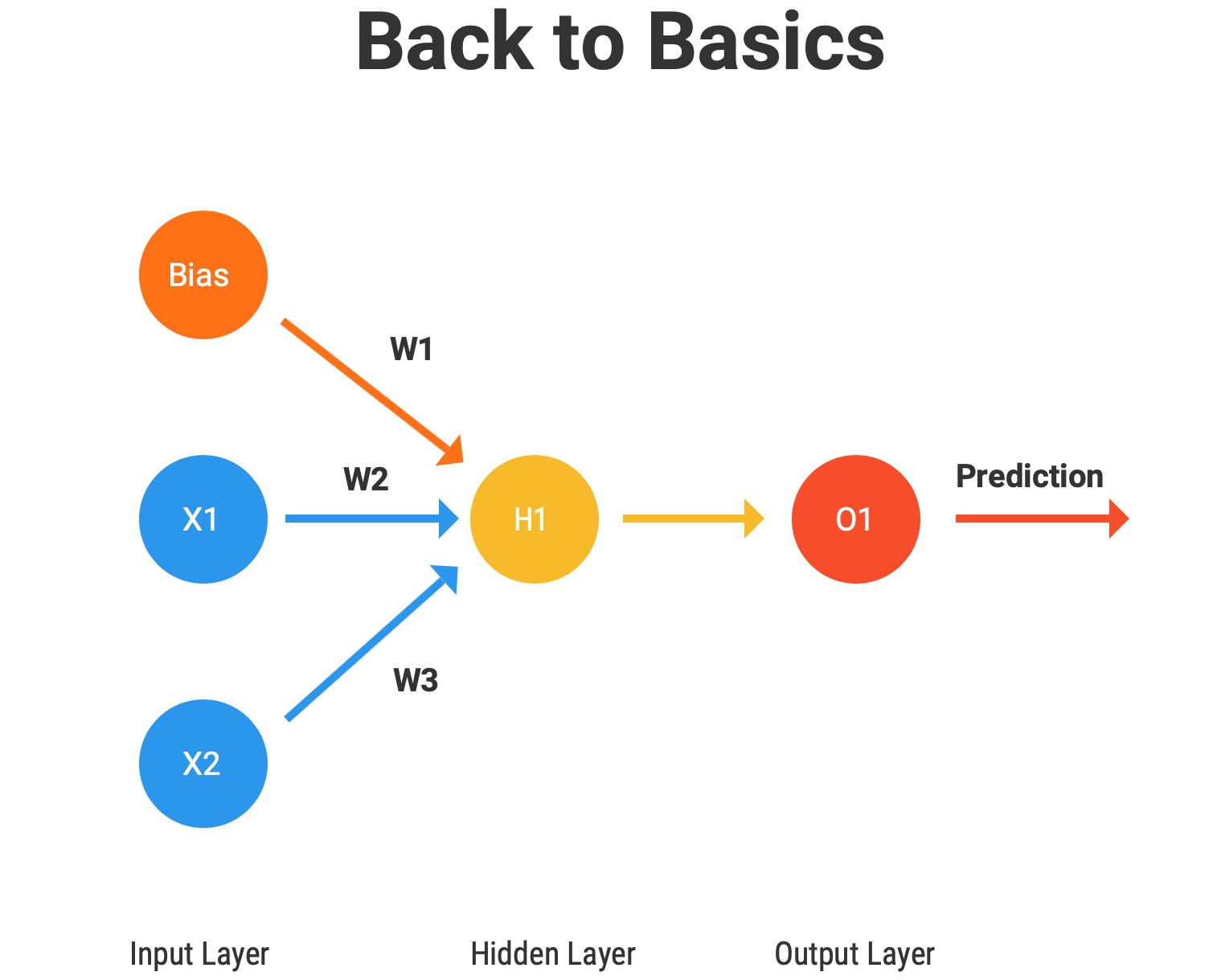
Pretty “basic” right? X1 and X2 are two neurons in the input layer, there’s one neuron, H1 in the hidden layer and lastly, we have the output neuron, O1. Each connection has a weight associated with themselves (W1, W2, W3) and for simplicity, we’ve assumed the output of the H1 neuron is our prediction which is represented by the O1 neuron. Also, don’t miss the bias unit!
It’s time for some math! Bring up the Forward Pass, please!
The Forward Pass.
Again, the forward pass is pretty straightforward. We’ll go layer by layer.
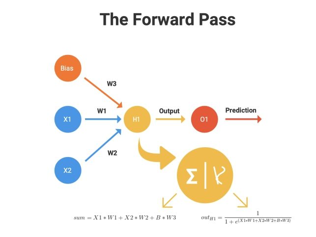
1. The value in the input neurons, X1 and X2, gets multiplied by their respective weights (W1 and W2) and is sent to the input of the hidden layer neuron H1 along with the product of the bias and its associated weight (W3).
2. At the hidden layer, two key operations are performed, summation and transformation.
2.1. A summation is just the addition of all that is incoming (X1*W1, X2*W2 and B*W3, where B is the bias value).
Transformation is where we use the “Activation Function” to apply a non-linear transformation to the output obtained in the summation. We’ll assume the sigmoid activation for our brief discussion here which is given by the formula:
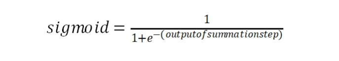
3. Once the transformation is applied, the output is sent to the output layer neuron (O1) as a prediction.
The forward pass can be thus summarised as in Fig 4 below:
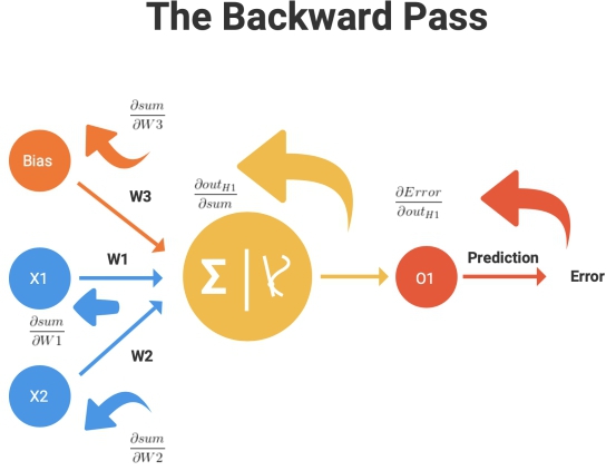
The Backward Pass.
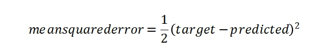
The backward pass is where the magic happens. The fundamental concept is to adjust the weights (W1, W2, W3) such that our predicted value is closer to the target value. From here, originates the concept of a “loss” function. For our example, let’s assume the loss function to be the mean squared error between the target and our prediction which is given by the equation:
This is where our backward pass begins. Our objective now is to minimize this loss function. How do we do that? Well, imagine this, if you were in front of multiple slides, all with different slopes and your objective was to get to the bottom as fast as you can, which slide would you choose? The one with the steepest slope of course!
Here, the loss function is analogous to our various slides and we need to get to the lowest possible value (our objective is minimization, after all!). And how do we calculate the “slope” of something in mathematics?
Enter Gradients!
Let’s go layer by layer, starting backward, from the output layer.
Now the training process begins to make a whole lot of sense, but, what was the point of this discussion?
Well, you see, unfortunately for our “Back to Basics” Neural Network, it will never make it out of this toy example. A simple Neural Network was intentionally chosen so that the forward pass and backward pass mechanisms can be delineated clearly. In reality, when solving actual industry problems, such Neural Networks never make it out of textbooks and that’s the whole point of this! The forward pass is fairly easier to compute. But you can imagine how complicated the backward pass would get to calculate if we began to increase the size of our Neural Network! If it’s hard imagining the calculations needed for even a10 hidden layers deep Neural Network, try imagining it for a 152 layer deep Neural Network! And wait for it! That’s not all! The 152 layer deep Neural Network we asked you to imagine, is the ResNet, which was the state-of-the-art….. 5 years ago.
It is thus, that the need for automatic differentiation is born, to keep track of all the gradients being propagated. PyTorch’s torch.autogrod module does exactly this. It abstracts the complicated mathematics and helps us calculate gradients of high dimensional curves with only a few lines of code. We’ve had enough of theory! Let’s jump to some code now!
Finally, the CODE!
The way we left off in the previous blog, we learned how to define tensors in PyTorch. Now, we’re going to look at another attribute of all tensors defined in PyTorch, called grad_fn. This attribute, along with torch.autograd, holds the gradient of the defined tensor as it moves through operations and network layers.
First, we’ll define some tensors, like we did last time, with a slight change.
import torch

a = torch.randn((3,3), requires_grad = True)
Notice something? On setting requires_grad = True, PyTorch starts forming a backward graph that tracks every operation applied to them to calculate the gradients. requires_grad is contagious. It means that when a tensor is created by operating on other tensors, the requires_grad of the resultant tensor would be set True given at least one of the tensors used for creation has its requires_grad set as True.
Let’s go ahead and see how this works.
w1 = torch.randn((3,3), requires_grad = True)
w2 = torch.randn((3,3), requires_grad = True)


d = w1*a + w2*a

E = 10 - d

print("The grad fn for d is", d.grad_fn)
If you run the code above, you get the following output:
Out:
The grad fn for d is <AddBackward0 object at 0x1213afc48>
A couple of points to note here:
- d is our Tensor here. It’s grad_fn is <ThAddBackward>. This is basically the addition operation since the function that creates d, adds inputs.
- The backward function of the <ThAddBackward> basically takes the incoming gradient from the further layers as the input. What autograd does for is that the gradient of E w.r.t to d and is stored in grad attribute of the d. It can be accessed by calling d.grad.
Now since we understand what autograd is and how it works, let’s go on to the next module we’ll be needing, torch.nn
The NN Module.
The functionality of torch.nn module is a lot like the tensorflow.keras.layers class in that if offers out-of-the-box layer wrappers for us to use for building our network. It is also a lot like tensorflow.keras.Model in that it offers the functionality to further wrap those layers into a single “model”.
Once again, nothing quite teaches like an example, so let’s see this in code and build our very first Neural Network in PyTorch!
Our First Neural Network in PyTorch!
Since the readers are being introduced to a completely new framework, the focus here will be on how to create networks, specifically, the syntax and the “flow”, rather than on building something complex and closer to the industry, which might lead to confusion and result in some of the readers not exploring PyTorch at all.
Y’all will need time to digest this. So we’re going to take it slow. Let’s begin!
Step I. As always, the necessary imports!
Pretty much the stuff we talked about in this blog, along with some standard stuff with the exception of torch.optim. Remember we said this is the third important module we’ll be required to build the Neural Network? Nothing too complex about it though. It’s equivalent to the tensorflow.keras.optimizers which provides out-of-the-box optimizers to use such as SGD, Adam, RMSProp and the likes. Hold on, we’ll see this in action real soon!
import torch
from torch import nn
from torch import optim
Import numpy as np
Step II. Generate some data!
Neural Networks literally fall flat on their face without data, so let’s generate some data that we’ll be using to train on.
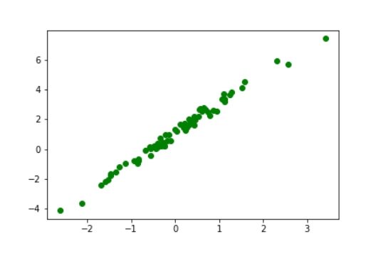
# Ensure Reproducibility
torch.manual_seed(0)

# Data Generation
x = torch.randn((100,1), requires_grad = True)
y = 1 + 2 * x + 0.3 * torch.randn((100,1), requires_grad = True)

# Shuffles the indices
idx = np.arange(100)
np.random.shuffle(idx)

# Use first 70 random indices for train
train_idx = idx[:70]
# Uses the remaining indices for testing
test_idx = idx[70:]

# Generates train and validation sets
x_train, y_train = x[train_idx], y[train_idx]
x_test, y_test = x[test_idx], y[test_idx]
The data we’ve generated looks like this:
Step III. Build the Network!
In PyTorch, every Neural Network that we define, will be as a class and that class will ALWAYS have these two mandatory functions, __init__() and forward().
class OurFirstNeuralNetwork(nn.Module):
# The __init__() function defines the architecture.
def __init__(self):
super(OurFirstNeuralNetwork, self).__init__()
# Here we "define" our Neural Network Architecture
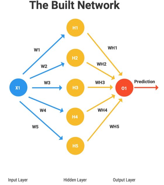
# We will define the first layer to have 5 neurons with one input (since our input is a point)
self.fc1 = nn.Linear(1, 5)
# Apply transformation (ReLU)
self.non_linearity_fc1 = nn.ReLU()
# We will define the output layer to have 1 neuron with 5 inputs (from the previous 5 neurons)
self.fc2 = nn.Linear(5,1)
# Checkout Fig. 8 to see what we just created!
# The forward() function defines the forward pass.
def forward(self, x):
# Here we define how activations "flow" between neurons. We've already discussed the "Sum" and "Transformation" steps of the forward pass.
sum_fc1 = self.fc1(x)
transformation_fc1 = self.non_linearity_fc1(sum_fc1)
out = self.fc2(transformation_fc1)
return out
# Get the model to proceed for training
model = OurFirstNeuralNetwork()
The Tensorflow (Keras) equivalent of this would be like so:
# Define the input layer

input_layer = Input(shape=(1)


# Define the model architecture

fc1 = Dense(5, input_shape=input_shape)(input_layer)
non_linerarity_fc1 = ReLU()(fc1)
out = Dense(1)(non_linerarity_fc1)


# Get the model to proceed for training

model = Model(inputs=input_layer, outputs=out)
It’s easy to verify, since most of our readers are familiar with Tensorflow (Keras), that the built network here is also exactly like Fig. 8!
Step IV. Time to “Torch” it!
This is where it all comes together folks! All our previous discussions on the forward pass, the backward pass, and the weight updates (to reduce the error) will finally bear fruit here and completely clear all your doubts regarding PyTorch training, conceptually and syntactically!
n_epochs = 100

# Define the loss function
loss_fn = nn.MSELoss(reduction=‘mean')

# Here we finally use the torch.optim module to initialise our optimiser!
optimizer = optim.Adam(model.parameters(), lr=1e-1)

# The training loop
# This where our prior discussion on forward and backward passes will help!

for epoch in range(n_epochs):

    model.train()
    prediction = model(x_train)
    loss = loss_fn(y_train, prediction)
    print(epoch, loss)
    loss.backward(retain_graph=True)
    optimizer.step()
    optimizer.zero_grad()
Let’s break the training loop part down and go over it line by line
- First, model.train(). A little counter-intuitive since we’ve been used to Tensorflow (Keras), but this does absolutely nothing except getting the defined model in “training mode”.
- Second, we do a forward pass with our data, x_train with model(x_train) and store the prediction.
- Third, we calculate the loss function, in this case, mean squared error.
- Next, we do the backward pass (backpropagation) with loss.backward() and computes the gradient of loss w.r.t to our weights.
- And lastly, optimizer.step() performs a parameter update based on the current gradient and the update rule.
- optimizer.zero_grad() is just to flush out the gradients calculated in this iteration and start fresh in the next one!
See? We told you everything would come together at the end of this blog!
True to our Model Life-Cycle diagram (Fig. 1), Step IV in Tensorflow (Keras) is a breeze though.
model.compile(optimizer=‘adam', loss='mse')
model.fit(x_train.detach().numpy(), y_train.detach().numpy(), epochs=100)
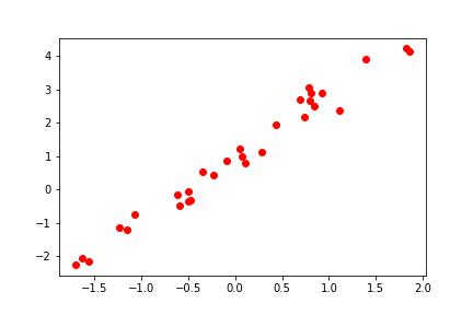
Here is a plot of the predictions after our model finishes training:
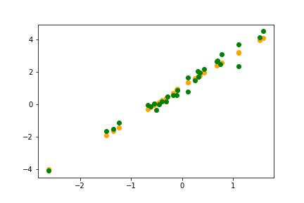
Not bad at all! Our very simple Neural Network has picked up the data distribution very well indeed!
Concluding Thoughts.
At the very beginning, we talked about the Tensorflow (Keras) “Flow” and its “Model Life-Cycle”, well, it’s only fitting that we conclude with the PyTorch “Flow” summarized in Fig. 9.
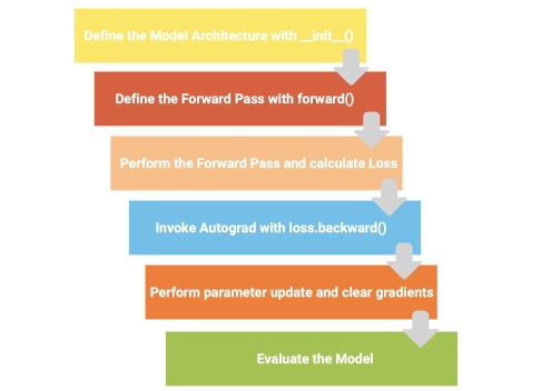
In the forthcoming blogs from this series, we’ll be doing a bunch of other cool stuff using actual data and way more complex architectures but this “flow” of how we go about things in PyTorch, will essentially be the same and we hope the readers have taken into it! Until next time!
More From The Series:
#1. PyTorch: The Dark Horse of Deep Learning Frameworks (Part 1)
#2. The Next Step: Building Neural Networks with PyTorch (Part 2)
#3. Marching On: Building Convolutional Neural Networks with PyTorch (Part 3)