

“I get very excited when we discover a way of making neural networks better – and when that’s closely related to how the brain works.”
Geoffrey Hinton
The Connection
Perhaps, the reason why convolutional neural networks have, time and again, proved themselves to be so adept at myriad vision tasks, is because they take their inspiration from one of the most evolved biological systems that exist today – the human visual system.
Not surprisingly, Convolutional Neural Networks or CNNs were not the first class of models conceived to emulate the architecture of our visual system. Various such neurocognition models exist in the literature today. However, it’s one thing to take inspiration from something, another thing to actually get it to work.
CNN was not the first model mimicking the human visual system, but it was the first model that came the closest to human-level performance, and in fact, as of this writing, has also beat human benchmarks in some vision tasks already.
The reason for their ridiculously widespread success, apart from being biologically inspired, can be attributed to the fact that among all its neurocognition predecessor models, CNNs produced activity that directly corresponded to the activity of different areas in the human visual system. This finding has been further strengthened with the introduction of Deep CNNs, where later layers in the network are noted to be in correspondence to later areas in the ventral visual stream.
A bit of medical jargon there, but the point being made, is that CNNs are both, architecturally and functionally similar to our own visual system.

Read More On Convolutional Neural Networks:
The Fundamentals
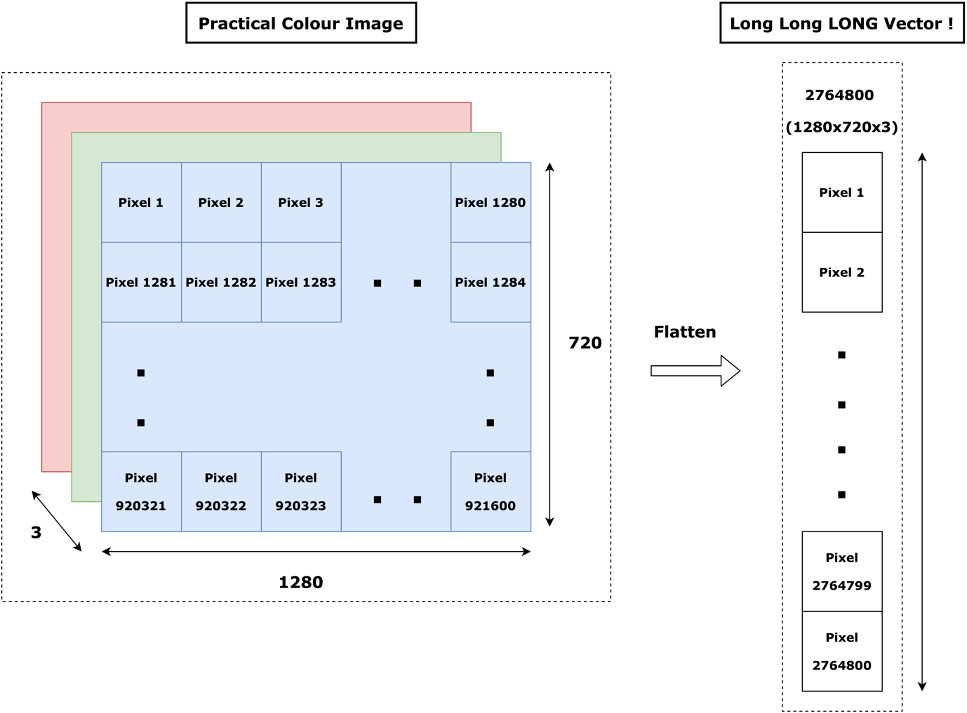
The traditional way to deal with image data (2D) before CNNs really came to the scene, was by flattening images to one long sequence (1D) and passing it to a Deep Neural Network or DNN. This worked quite well for small binary images (images without color information) but the inherent inefficiency in this approach presented itself when it was exposed to more real-world images with color depth (RGB channels) as shown in Fig. 1 and Fig. 2.
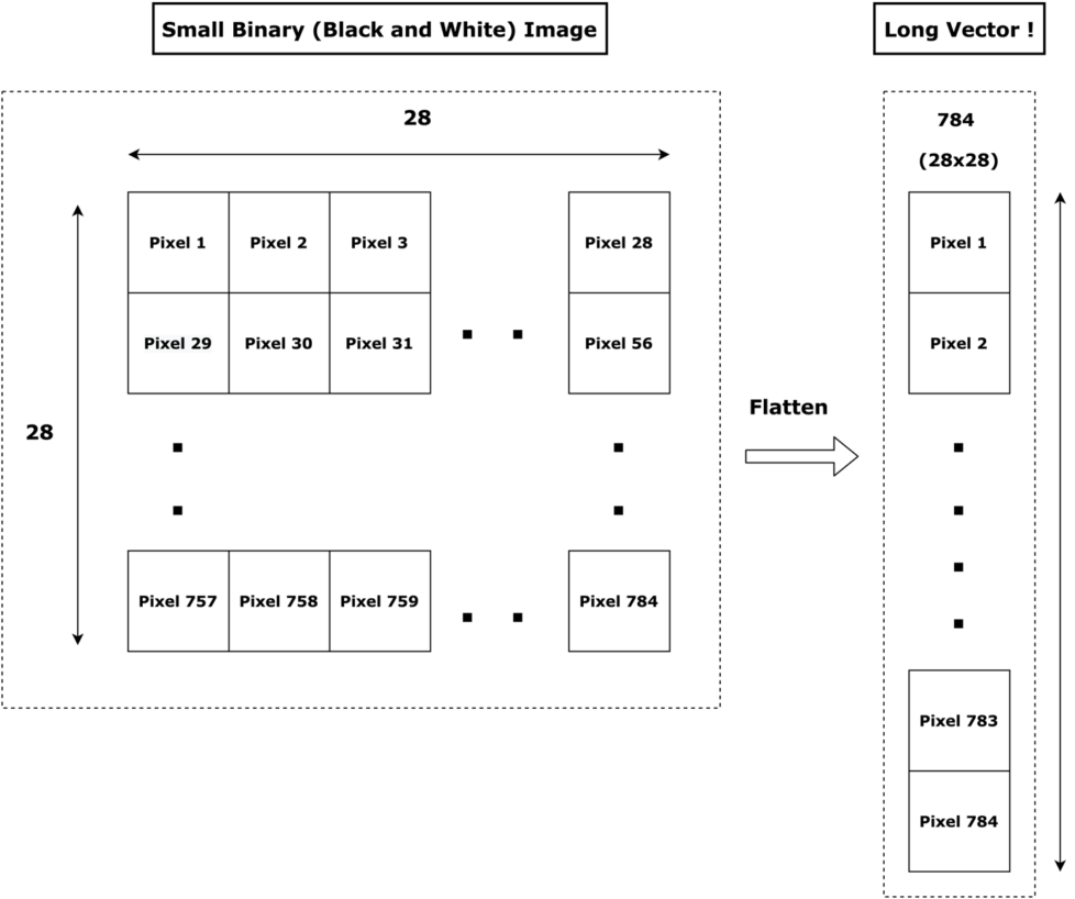
When the dimensions of the image are of a toy case, 28 x 28, the flattened vector (1D) is of length 784. That’s pretty doable!
However, when we take practical problem images, say, like the images captured by a car in an autonomous driving application, the length of the flattened vector almost touches three million!
Not only this, but the flattened (1D) vector does not retain any of the spatial or color information of the original image as shown clearly in Fig. 2!
Clearly, this approach is not scalable!
So the concept is this, how about we just let image data be a 2D sequence instead of all the fancy reshaping?
Drumrolls! Enter Convolutional Neural Networks!
Convolutional Neural Networks accept an image as a 2D sequence (that is, they accept an image as it is), and are thus capable of exploiting an image’s spatial structure and its color information, making it possible for these networks to extract deeper semantic features than an ordinary Deep Neural Network ever would.
The Power of Convolutions
A Convolutional Neural Network works on the principle of ‘convolutions’ borrowed from classic image processing theory.
Let us take a simple, yet powerful example to understand the power of convolutions better.
Imagine if you were tasked with ‘coaching’ a neural network to differentiate between the digits, ‘1’ and ‘2’. Also, you are given the ability to ‘talk’ to a neural network to guide it in this process! What would you advise that the network do?
Well, you would probably tell that the network that the digit ‘1’ has a characteristic feature – a vertical straight line; but the digit ‘2’ doesn’t! Elegant!
However, the problem is, how would your network identify a vertical straight line?
The answer is through convolutions!
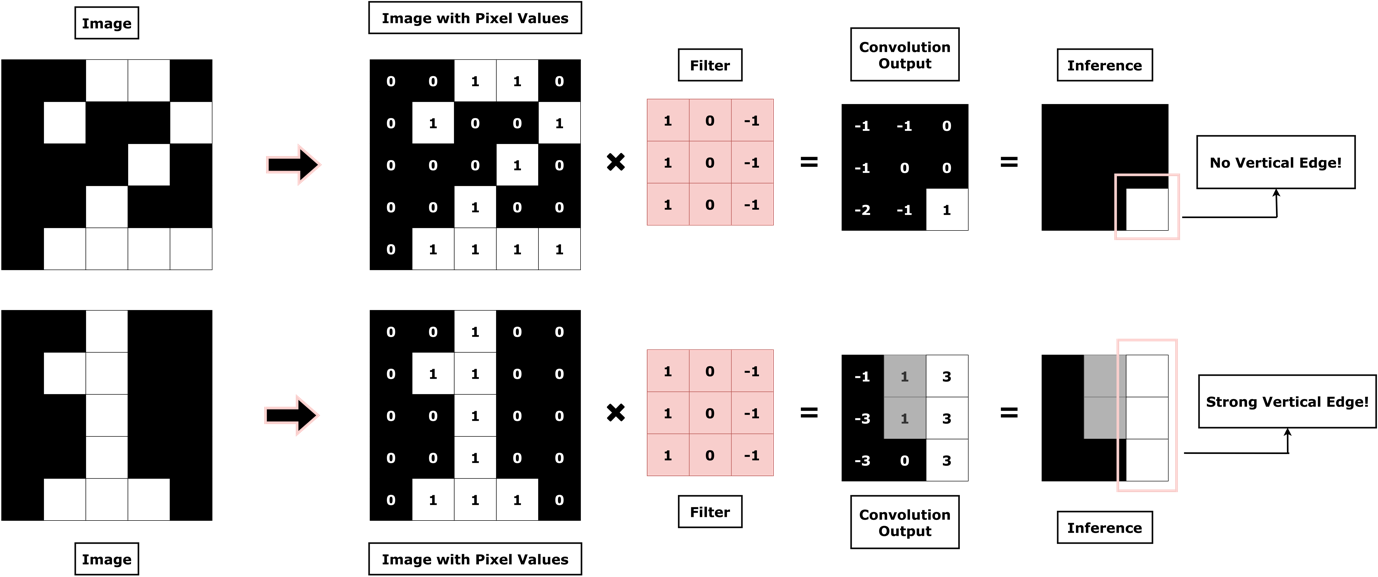
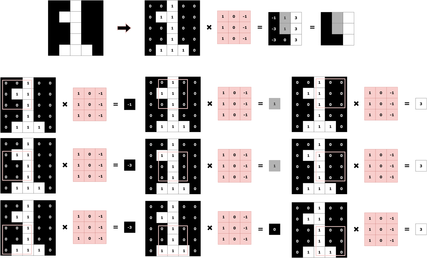
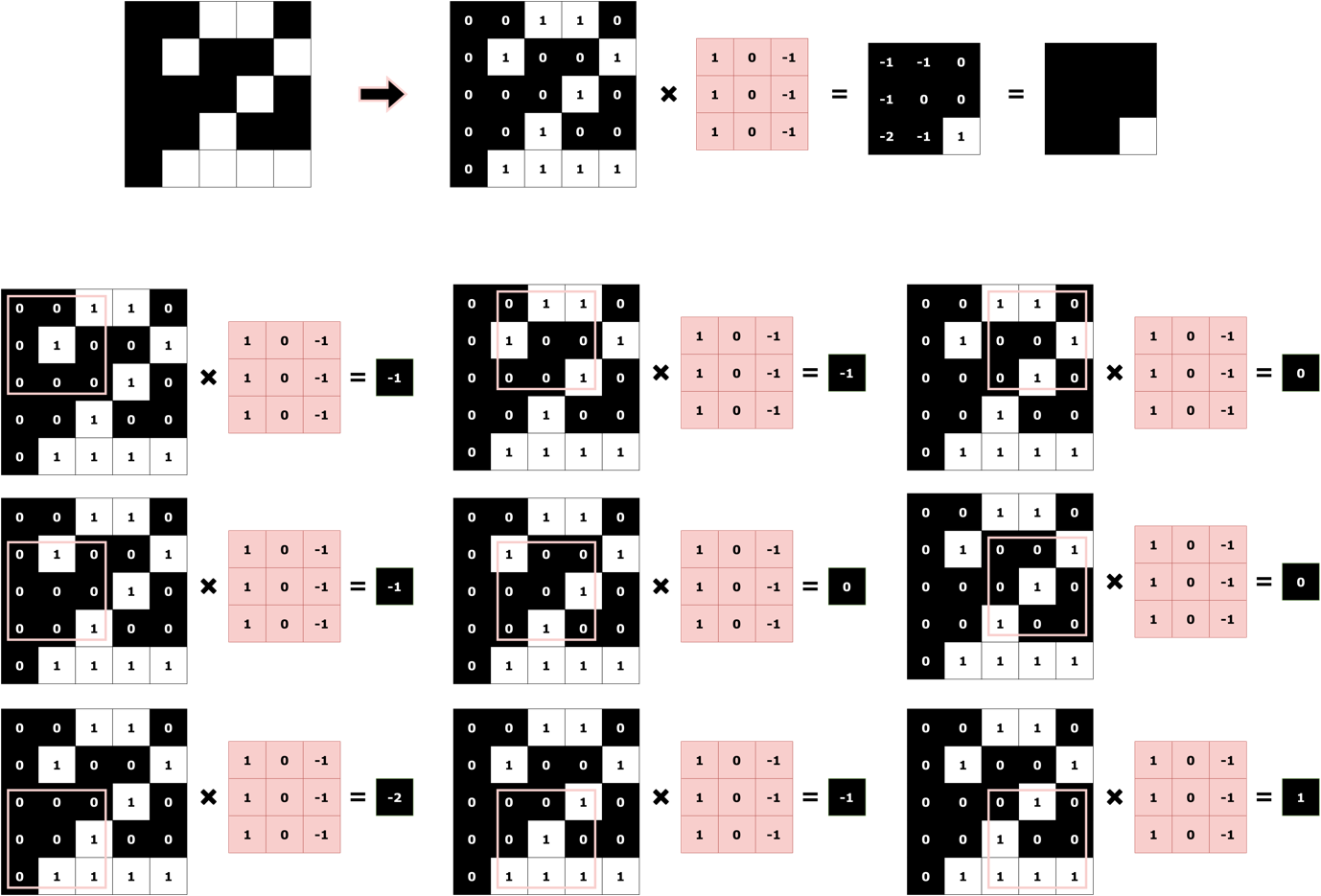
Fig. 3 shows how using convolutions with the right filter, a vertical edge in an image can be correctly identified. The convolution operation is an element-wise dot product, followed by summation as illustrated in Fig. 4 and Fig. 5 for both the digits, ‘1’ and ‘2’.
Of course, in this example, you smartly chose a filter for the network which would detect vertical edges in the image. But you aren’t going to be around forever. This means, your network needs to learn the filters that are optimal for solving a given task by itself! And the good news is, they do – through backpropagation.
In a nutshell, Convolutional Neural Networks start off by randomly initializing filters (like the one you chose, but many more) and in the process of training (backpropagation), they keep modifying the initialized filters such that the given task can be accomplished.
For this example task, you’d expect your CNN to ‘learn’ the filter that detects a vertical straight line through backpropagation and become really good at classifying the two digits apart from each other!
This toy example also helps us see how and why CNNs mimic our visual system which as we mentioned, is the reason for their stellar performances time and again!
In a real-world task though, your network would need many more filters than just one to actually get good at the given task, as we’ll shortly see when we code up our own CNN in PyTorch to classify fashion accessories!
We deliberately digressed from the code until now, because we wanted to introduce this topic to you with a little bit of background. AI has become such a fast-paced field that often learners tend to blindly jump straight to bits of ‘library’ code that does all the work for you, without first taking time with the fundamentals.
Remember, in AI, understanding the philosophy, background, and math of a particular architecture or technique, is as important as learning its execution in terms of code for long time success!
The PyTorch Flow.
Learners that have landed here from our previous two blogs, will be familiar to what we call the ‘PyTorch flow’ presented to you in Fig. 6. If you are a new learner, we highly recommend you go through the previous two blogs in this series and then come back here for the best possible learning experience!
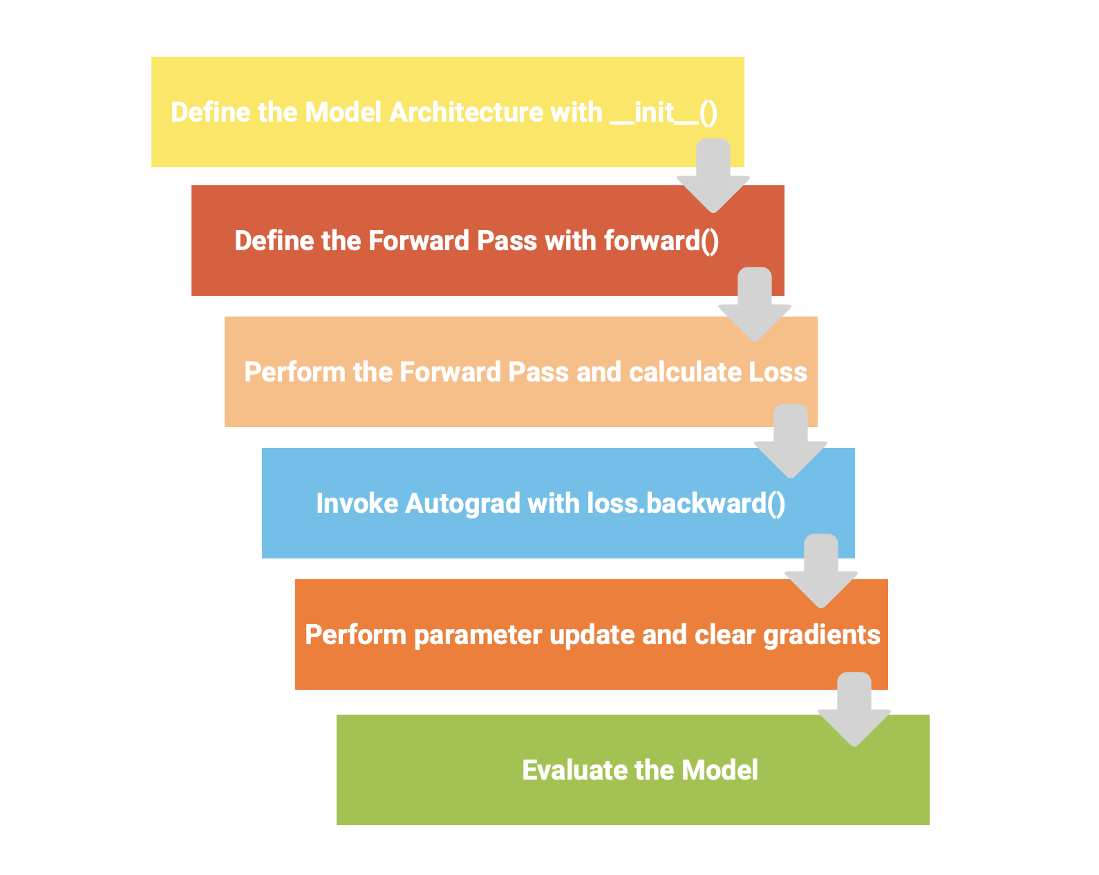
Fig. 6 illustrates the steps we’ll follow when building our own CNN for classifying fashion accessories.
More from the Series:
- PyTorch: The Dark Horse of Deep Learning Frameworks (Part 1)
- The Next Step: Building Neural Networks with PyTorch (Part 2)
Oh wait, did we introduce you to the data yet?
The Fashion MNIST Dataset
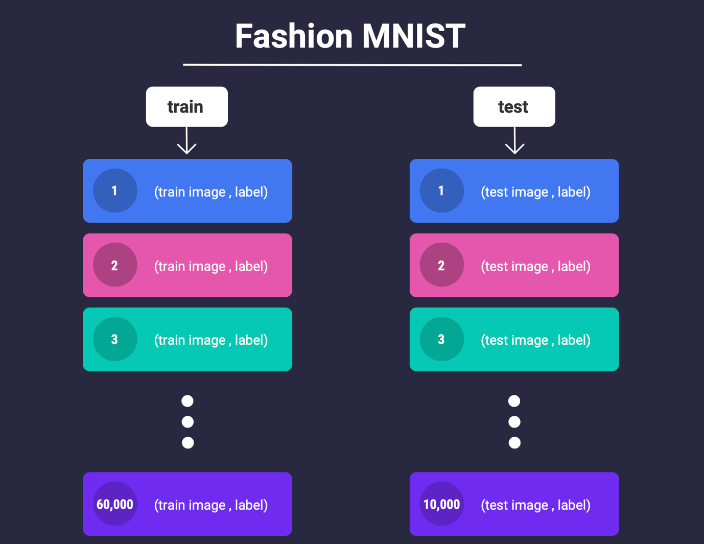
Fashion-MNIST is a dataset of Zalando’s article images consisting of a training set of 60,000 examples and a test set of 10,000 examples. Each example is a 28×28 grayscale image, associated with a label from 10 classes (Rasul and Xiao).
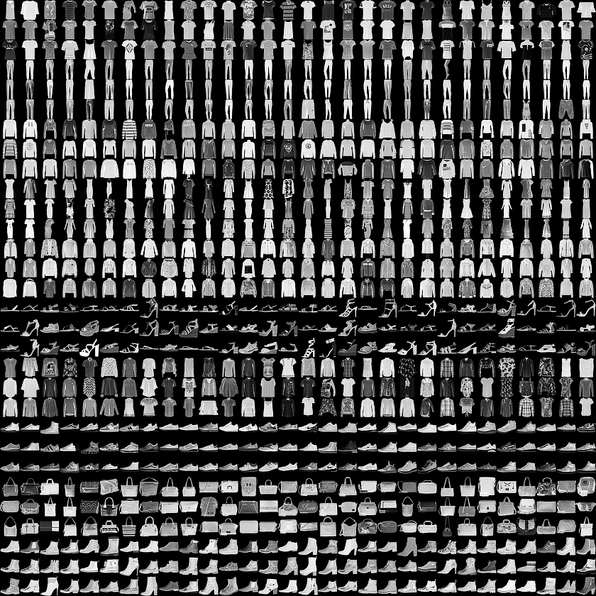
Fig. 7 below is a small snapshot of the dataset with each class taking three rows.
Further, we have created a Table. 1 to clearly list all the 10 classes along with the labels.
| Class | Label |
| 0 | T-shirt/top |
| 1 | Trouser |
| 2 | Pullover |
| 3 | Dress |
| 4 | Coat |
| 5 | Sandal |
| 6 | Shirt |
| 7 | Sneaker |
| 8 | Bag |
| 9 | Ankle Boot |
Table 1. Classes and Labels of the Fashion MNIST
PyTorch’s torchvision library makes loading Fashion MNIST (along with other popular datasets) and pre-trained models like AlexNet and VGG seamless.
Let’s go ahead and import this module first, and then look at the code to load Fashion MNIST.
Also Read: Build your own handwritten digit recognition system using MNIST dataset in Python!
Loading the Fashion MNIST Dataset
First, of course, we need to install the torchvision library on our machine. This can be done with the following command:
(Using pip)
pip install torchvision
(Using conda, if have Anaconda on your machine and prefer it)
conda install -c pytorch torchvision
(Using an IDE or an IPython interface, such as Jupyter Notebooks)
!pip install torchvision
Although we highly recommend that you don’t try to run this on your local machine and instead, opt for a cloud-hosted runtime like Google Colaboratory Notebooks!
There are several reasons for you to make the switch to Colab:
- A cloud-hosted runtime lets you forget about heating up your machines during neural network training and avoid ‘library’ clutter!
- The power of GPU is available to you for accelerating training.
- Great for rapid experimentation and learning new things (like coding up CNNs in PyTorch!)
- It has popular libraries including torchvision preinstalled!
- Naturally comes with the full power of Jupyter Notebooks which lets you add text cells, images, and more along with code!
And the absolute finisher:
- It is completely free of cost!
To facilitate your switch, we have gone ahead and curated a fully functional Colab Notebook for this tutorial which you can follow alongside, or check out later!
We’ll put the link here below:
Note how we don’t have to install any of the libraries in the notebook!
Torchvision installed, we are now ready to import it with a simple import as shown:
import torchvision
import torchvision.transforms as transforms
import torch
from torch.utils.data import DataLoader
You’ll note that along with torchvision, we’ve also imported several other modules. It will make perfect sense to you in a bit. But first, let us see the code for downloading Fashion MNIST and loading it, which is literally two lines!
# Load the Train and Test sets

train = torchvision.datasets.FashionMNIST(root='FashionMNIST/',
train=True,
download=True,
transform = transforms.ToTensor())

test = torchvision.datasets.FashionMNIST(root='FashionMNIST/',
     train=False,
     download=True,
     transform =
 						     transforms.ToTensor())
Here’s the thing, Fashion MNIST stores the train and test images in the PIL format by default. But we know that if we want to be able to do any computation on those images, we need to convert it to a torch tensor which is exactly why the transform = transforms.ToTensor() argument comes into the picture!
Once the train and test sets are loaded, it always helps to visualize how the variables train and test actually hold the data as shown in Fig. 8. In our notebook, we have also provided a small code snippet that will strengthen your understanding of how data is held in the train and test variables. Do check it out!
We can also print off the lengths of train and test to confirm that all is as per expectation:
# Confirm that we have the Train and Test sets as expected

print('Length of training set: {}'.format(len(train)))
print('Length of test set: {}'.format(len(test)))

Output:

Length of training set: 60000
Length of test set: 10000
What we’ll do next, is that we’ll create batches of 32 within the train and test data along with their labels. This is where the imported DataLoader class from torch.utils.data can help us!
The below code snippet uses the DataLoader class that takes our train and test variables and returns a batched version of the images held in it, in sizes of 32.
We store this batched version of our train and test data in two new variables, train_data_loader and test_data_loader
# Create batches of size 32 within the train and test datasets

train_data_loader = DataLoader(train, batch_size=32, shuffle=True)

test_data_loader = DataLoader(test, batch_size=32, shuffle=False)
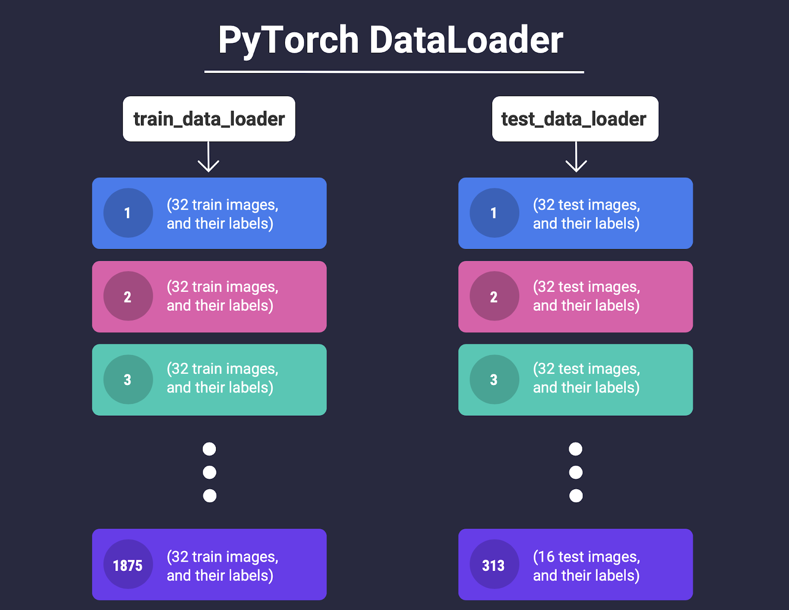
We show this batching process with the help of a conceptual visualization in Fig. 9.
Now each datapoint in the train_data_loader and test_data_loader is a batch of 32 images along with their labels.
A quick sanity check tells us this is indeed the case since 60000/32 = 1875 matches with the length returned by calling len()on train_data_loader!
# Sanity check to verify that the data has been batched in sizes of 32

len(train_data_loader)

Output:

1875
(Note that for the test set, 10000/32 is 312.5 which means only 16 images can be put in the last batch, as shown in Fig. 9. See if you can verify this in code in our notebook!)
Let’s quickly see some examples of the data we have!
import numpy as np
import matplotlib.pyplot as plt

# Get some random training images
data_iter = iter(train_data_loader)
images, labels = data_iter.next()


# Function to show some images from the dataset
def imshow(img):
    npimg = img.numpy()
    plt.imshow(np.transpose(npimg, (1, 2, 0)))
    plt.show()

# Show images
imshow(torchvision.utils.make_grid(images))

# Print labels
classes = ('T-Shirt/Top', 'Trouser', 'Pullover', 'Dress','Coat', 'Sandal', 'Shirt', 'Sneaker', 'Bag', 'Ankle Boot')
print(' '.join('%5s' % classes[labels[j]] for j in range(4)))

Output:
Model Architecture and Forward Pass
The first two steps according to Fig. 6 are defining model architecture with __init__() and the forward pass with forward()
import torch.nn as nn
import torch.nn.functional as F

class Net(nn.Module):

    # The __init__() function defines the architecture.
    def __init__(self):
        super(Net, self).__init__()
        self.conv1 = nn.Conv2d(in_channels=1,
  out_channels=16,
  kernel_size=3)
        self.conv2 = nn.Conv2d(in_channels=16,
                               out_channels=16,
                               kernel_size=3)
        self.pool1 = nn.MaxPool2d(2, 2)
        self.conv3 = nn.Conv2d(in_channels=16,
                               out_channels=32,
                               kernel_size=5)
        self.conv4 = nn.Conv2d(in_channels=32,
                               out_channels=32,
                               kernel_size=5)
        self.pool2 = nn.MaxPool2d(2, 2)
        self.fc1 = nn.Linear(32 * 5 * 5, 256)
        self.fc2 = nn.Linear(256, 128)
        self.fc3 = nn.Linear(128, 10)

    # The forward() function defines the forward pass.
    def forward(self, x):
        x = F.relu(self.conv1(x))
        x = F.relu(self.conv2(x))
        x = self.pool1(x)
        x = F.relu(self.conv3(x))
        x = F.relu(self.conv4(x))
        x = self.pool2(x)
        x = x.view(-1, 32 * 5 * 5)
        x = F.relu(self.fc1(x))
        x = F.relu(self.fc2(x))
        x = self.fc3(x)
        return x

OurFirstCNN = Net()
We have already covered all the syntactical elements of __init__() and forward() in our previous blog so we’ll just be going over the parts that are different.
1. nn.Conv2d(): Defines a convolutional layer for us by taking in three key arguments, in_channels, out_channels, and kernel size.
-
in_channels: Here we define the number of channels the input image to this layer is going to have. In our example, for the first convolutional layer,in_channels = 1, because all our images in the dataset are grayscale.
-
out_channels: Number of filters (or kernels) that you want to initialize for the given layer.
Note, technically this argument specifies the number of channels produced by the convolution, but that is always equal to the number of filters anyway, so we find our alternate definition a little easier to think of than the former.
-
kernel size: As straightforward as they come, this argument specifies the size of our filter (or kernel). Usually, a good size is between 3×3 to 7×7.
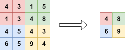
2. nn.MaxPool2d(): This implements the simple ‘pooling’ operation, an example of which is shown in Fig. 10. As an argument, it takes the factor by which to reduce dimensionality along the axes of a convolved image. Essentially, it performs downsampling by preserving only the maximum activations.
A small point that needs a little discussion is the line:
x = x.view(-1, 32 * 5 * 5)
Recall that if we want to pass a 2D sequence to a fully connected layer (specified by nn.Linear), we must flatten it to a 1D sequence. After passing through several convolutional layers, the image is essentially converted to what is called a ‘feature map’. This feature map is of considerably higher dimensionality than the original image. For our example, the image has 1 channel at the beginning but ends up being compressed into a ‘feature map’ having 32 channels!
At this point, enough features have been extracted by the filters that acted on the image through convolution, in all the layers that the image went through. And now that the features have been extracted, it would be fair to flatten it to a 1D sequence and leave the classification to a Deep Neural Network or DNN which is exactly what x.view(-1, 32 * 5 * 5) does – a simple flattening operation.
Our Colab Notebook has some more code snippets that clearly demonstrate the behavior of the x.view()function. Be sure to check that out!
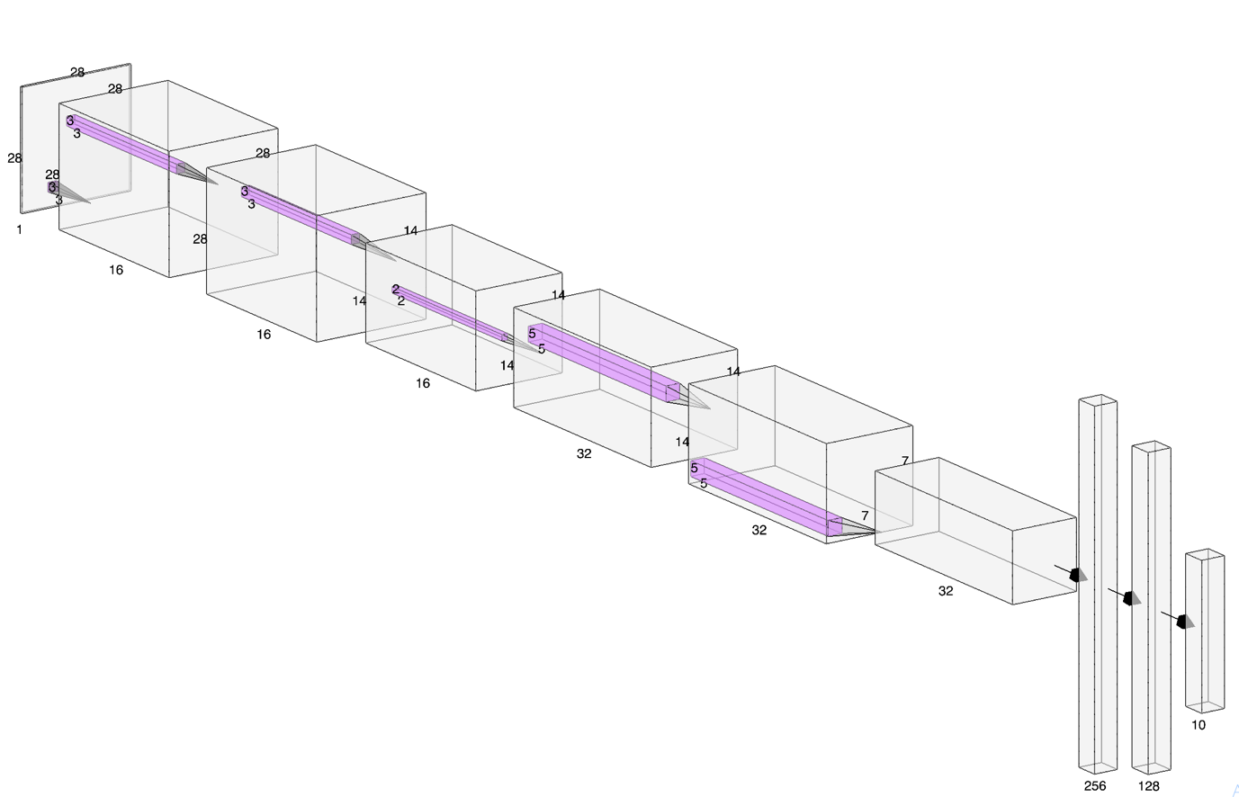
The architecture of our designed CNN is presented in Fig. 11.
We have also marked all the dimensions along with the filter and feature map sizes.
See if you can relate each block of the image to what we’ve coded in __init__()!
The Training Loop
From our developed ‘PyTorch Flow’ in Fig. 6, the next steps are as follows:
- Performing the forward pass and calculate the loss.
- Invoke Autograd to backpropagate.
- Use the optimizer to update the gradients.
If we repeat these three steps for all the images in a loop, what we’ll have, is the training loop! Pretty easy! Let’s jump to the code!
Or… maybe not.
To perform any of those steps, we would first need to define a loss function and an optimizer as follows:
import torch.optim as optim

# Define the loss function and optimizer.
# We define the crossentropy loss here because we have 10 classes
# Adam as optimizer with its default learning rate should work well
loss_fn = nn.CrossEntropyLoss()
optimizer = optim.Adam(OurFirstCNN.parameters(), lr=0.001)


# Define a function for calculating accuracy
def accuracy():
  correct = 0
  total = 0
  with torch.no_grad():
      for data in testloader:
          images, labels = data
          outputs = OurFirstCNN(images)
          _, predicted = torch.max(outputs.data, 1)
          total += labels.size(0)
          correct += (predicted == labels).sum().item()

  print('Accuracy of the network on the 10000 test images: %d %%' %
 (100 * correct / total))
We’ve also defined a function for calculating accuracy which will help us evaluate the performance of our model during training and after.
Okay, yes now we good.
Now let’s show you the code!
# The Training Loop

for epoch in range(10):  # loop over the dataset multiple times

    for i, data in enumerate(train_data_loader, 0):

        # get the inputs; data is a list of [inputs, labels]
        inputs, labels = data

        # zero the parameter gradients
        optimizer.zero_grad()

        # forward + backward + optimize
        outputs = net(inputs)
        loss = loss_fn(outputs, labels)
        loss.backward()
        optimizer.step()

        # print statistics (loss and accuracy) for each mini-batch
        print('[%d, %5d] loss: %.3f' %
                  (epoch + 1, i + 1, loss.item()))


print('Finished Training')
Here’s what’s happening in the training loop:
1. For each iteration over the training dataset:
-
- For each minibatch (32 images with their labels as stored in
train_data_loader):
- For each minibatch (32 images with their labels as stored in
-
-
- Load the minibatch. Images in
inputsand thelabelsin labels. - Calculate the loss by passing the minibatch to the network
- Backpropagate the error by
loss.backward() - Update the gradients by
optimizer.step() - Print the epoch number, current minibatch number, loss along with the test accuracy by calling the
accuracy()function defined before!
- Load the minibatch. Images in
-
In TensorFlow (Keras), you probably wouldn’t have to define a separate function for accuracy like we did with PyTorch. But part of the reason that makes PyTorch so popular, is how it is super flexible without being complicated!
What do we mean by that?
Well, say you want to check, at each epoch, how well the network is performing with respect to all the different classes and not just how it is doing overall!
You can do this by simply switching out the accuracy function we had defined with this definition and call it in the training loop:
def accuracy():

  class_correct = list(0. for i in range(10))
  class_total = list(0. for i in range(10))
  with torch.no_grad():
      for data in testload Let’s also show you er:
          images, labels = data
          outputs = net(images)
          _, predicted = torch.max(outputs, 1)
          c = (predicted == labels).squeeze()
          for i in range(4):
              label = labels[i]
              class_correct[label] += c[i].item()
              class_total[label] += 1

  for i in range(10):
      print('Accuracy of %5s : %2d %%' % (
          classes[i], 100 * class_correct[i] / class_total[i]))
Doing this is not at all trivial in TensorFlow since we cannot use native Python-like we did with PyTorch here. We’ll see more of this in the next blog of this series where we give you learners some final thoughts comparing both these deep learning libraries!
In fact, in our Colab Notebook, we have implemented the same network with detailed comments in TensorFlow so you can compare each step side by side!
Hey! But How Did Our Network Perform?
Well, pretty awesome actually.
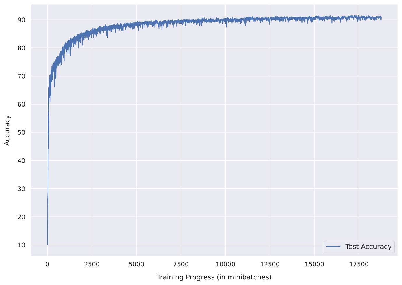
Take a look at the loss and accuracy graphs below in Fig. 12 and Fig. 13!
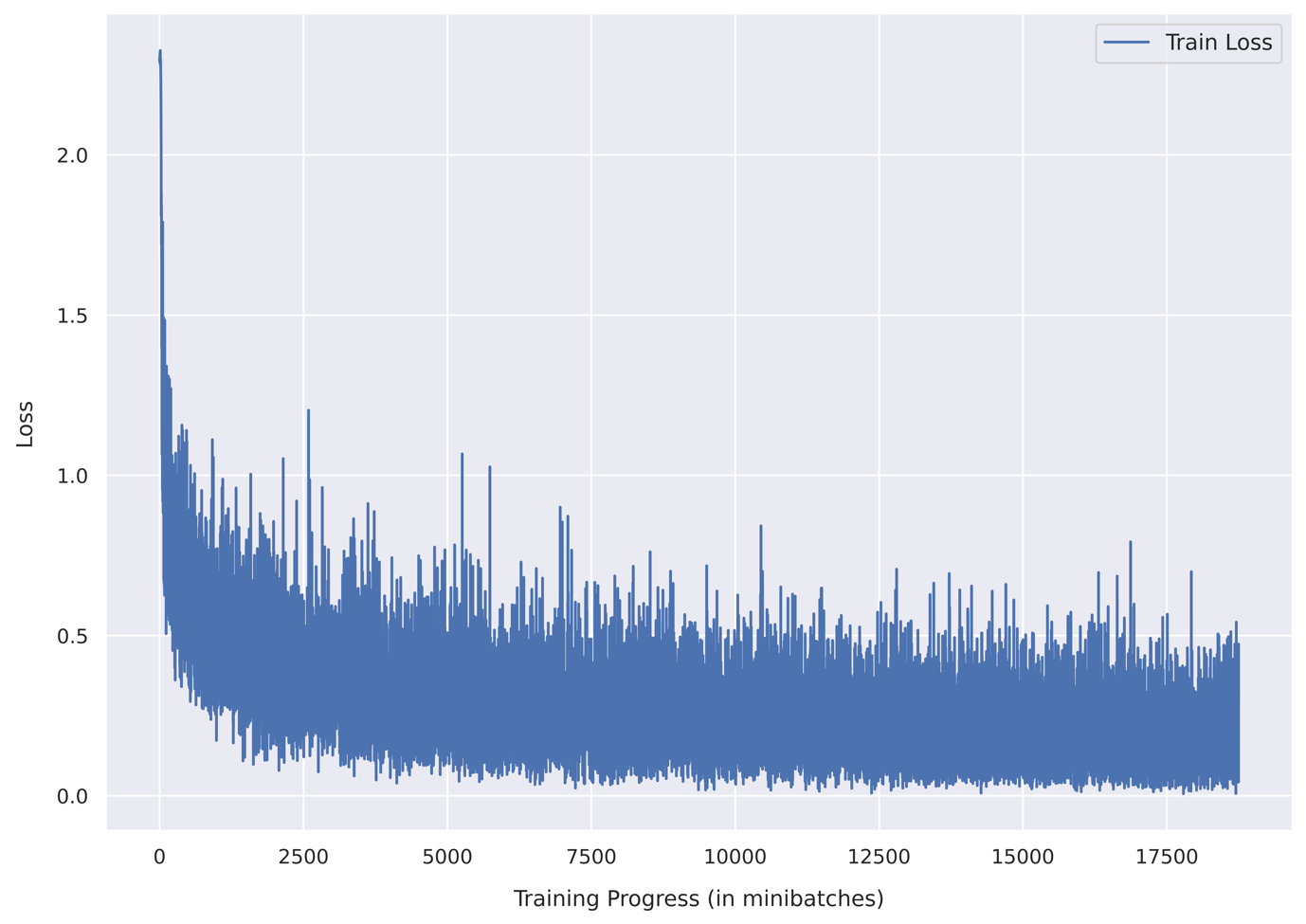
In just 10 epochs, we have achieved over 91% test accuracy! That’s super cool!
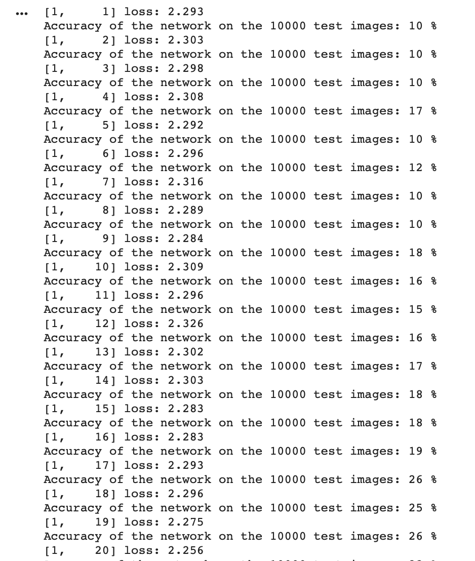
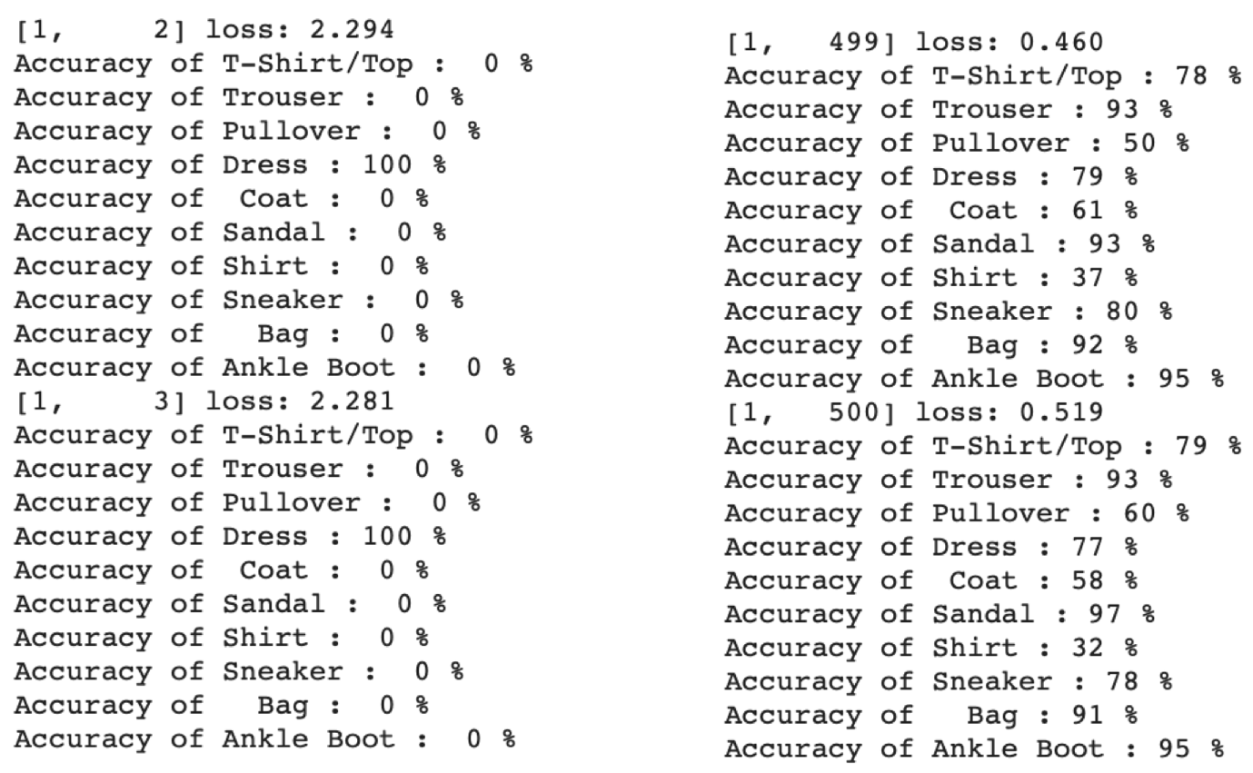
Let’s also show you how the console looks like when training, and also when we seamlessly switch out normal accuracy with a per-class accuracy! Check out Fig. 14 and 15!
Note from Fig. 15 that initially the per-class accuracy is 0% for almost all classes and it improves as the training progresses! Also, make a mental note of how insightful monitoring per-class accuracies can be!
Accelerating Training with GPU! ?
You’ll notice right away that the network takes quite a while to train. You can accelerate it by leveraging Colab’s free GPU (also the reason why we recommended Colab in the first place)!
To be able to use a GPU with PyTorch though, you need to ‘send’ your tensors ‘to the GPU’.
We’ve covered the syntax for how to do this in our first introductory blog on PyTorch. We’ve got you covered here, but if you haven’t read that blog, we suggest you head over there right away!
So all you really need to do is this:
1. Add these lines after the model definition, that is, after __init__() and forward():
device = torch.device("cuda:0" if torch.cuda.is_available() else "cpu")

# Assuming that we are on a CUDA machine, this should print a CUDA device:

print(device)

OurFirstCNN.to(device)
This selects the GPU so that PyTorch knows where to send your tensors.
2. Switch out the existing line in the training loop with:
# In the training loop

for epoch in range(10):  # loop over the dataset multiple times

    for i, data in enumerate(train_data_loader, 0):

        # Get the inputs
        inputs, labels = data[0].to(device), data[1].to(device)
This ‘sends’ your tensors ‘to the GPU’ we selected in the previous step. Note the .to(device) syntax!
3. Lastly, perform the same switch in our accuracy functions:
# In the accuracy functions

with torch.no_grad():

      for data in test_data_loader:

          images, labels = data[0].to(device), data[1].to(device)
Done! Your network will now train like a ?
Note that GPU training is the default behavior in our Colab Notebook! But we have provided options for you to do a CPU train too, just so that you can see the difference for yourself!
Your Learning Outcomes
- First, you learned the fundamentals of where CNN gets its superpowers from!
- Next, you explored the Fashion MNIST dataset and PyTorch’s DataLoader feature!
- Subsequently, we followed our ‘PyTorch Flow’ developed in earlier blogs to build a CNN step by step. We also touched on how flexible PyTorch can be when we seamlessly switched our accuracy functions to reveal more about our training!
- You learned how to accelerate network training by using Colab’s free GPU with PyTorch!
- In our Colab Notebook, you saw a step by step comparison of going about the same problem in PyTorch and TensorFlow!
Learners, apart from being one of the top all-time skills, coding is a very intricate field. And since not all the programming subtleties can be covered in a blog without the risk of it running too long, we’ve added lots of other supporting content in our Colab Notebook that will truly strengthen your understanding of not only PyTorch and how it compares to TensorFlow, but also Python coding in general!
Signing off here! Until we meet again!
More from the Series:
- PyTorch: The Dark Horse of Deep Learning Frameworks (Part 1)
- The Next Step: Building Neural Networks with PyTorch (Part 2)
Read More:
- Generative Adversarial Networks Series
- Understanding Computer Vision Techniques!
- DataOps: A Product of the Machine Learning Era

")


