
In the previous blog, we continued our deep dive into the world of Generative Adversarial Networks (GANs) with the pix2pix GAN which we also went ahead and coded up for ourselves. We achieved quite the results on the Maps to Google Maps problem statement where we attempted to convert a normal map to a Google Map UI which we’ve presented down below so that the reader can see it themselves.
Notice how the first image (from the left) in the middle row has more useful detail than the actual (target) Google Map image.
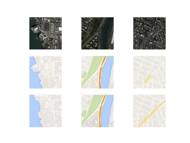
Top: Input Image; Middle: Generated Image; Bottom: Target Image.
At Eduonix, we curate all our blogs in such a fashion such that no blog is an absolute prerequisite to grasp the content of another blog because we believe it is unreasonable, on all levels, to expect the inquisitive reader to go through 4-5 blogs just so that they can understand the content of the blog they wanted to understand in the first place.
But for this GAN series, we do recommend all our readers who weren’t able to read the previous blogs (Introduction to GANs, pix2pix GAN), to go through it not because it is needed to understand this blog, but simply so that they can appreciate this blog and the subtle differences between the different types of GANs in general, better.
More from the Series:
- An Introduction to Generative Adversarial Networks- Part 1
- Introduction to Generative Adversarial Networks with Code- Part 2
- pix2pix GAN: Bleeding Edge in AI for Computer Vision- Part 3
- The Grand Finale: Applications of GANs- Part 5
GANs are, after all, the bleeding edge of AI.
That being said, as always, we’ll first talk a bit about Cycle GANs and introduce them to you, and then take up a coding example with a sample dataset so that the concept is crystal clear along with its applications.
Right so to kick things off, let’s just quickly summarise what we wished to accomplish with the pix2pix GAN.
With the pix2pix GAN, we undertook the image translation problem statement like the one we built the network for using the Maps Dataset (the results for which we’ve already shown at the beginning of this blog in Figure 1.)
The goal of the pix2pix GAN was to take an image of a map taken from a satellite and convert it to the all-familiar Google Maps UI.

A variety of other image translation tasks can be accomplished by the pix2pix GAN to great effectivity but there’s a certain caveat, a rather annoying one at that, which we need to vary of while using the pix2pix GAN for any specified task.
What is this caveat?
Actually, on second thoughts, we’ll have you try to figure it out.
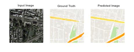
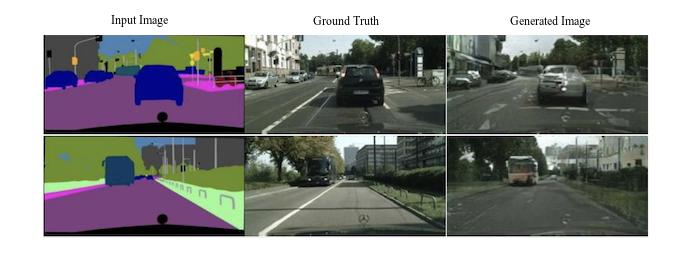
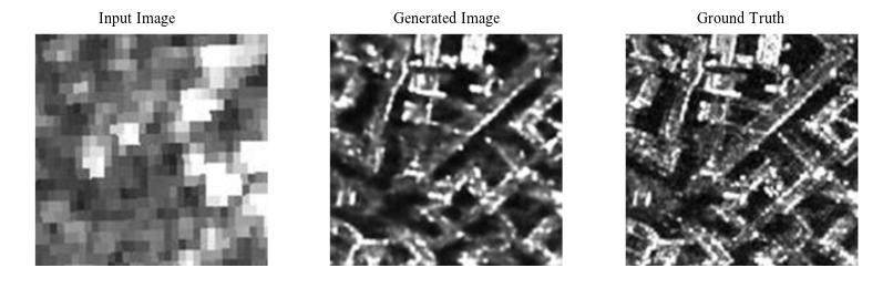
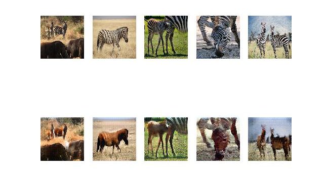
To point you in the right direction though, in the form of hints, we’ve provided sampled image trios (Input Image, Ground Truth and Generated/Predicted Image) of some tasks that have been performed rather well by the pix2pix GAN in the literature thus far.
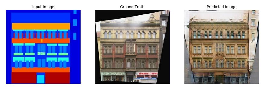
What do you see?
- truth. provided.
The Caveat.
A couple of observations to be with:
- The pix2pix GAN takes in an input image and uses the ground truth image to translate the input image to a closely matching desired image whilst retaining the structural information in the input image and infusing it with the style of the ground truth image. This we know from the previous blog as well.
- A second more interesting observation is that the Input Images and the Ground Truth Images are paired. This means the input image and the ground truth have the same exact structure, just different styles of representing the same objects or detail in the image. What do we mean by this? Well, consider the third example from the top. Notice that for a car in the input image there is a corresponding car in the ground truth of the translated domain at the exact same pixel positions as the car in the input image. This is true for every object in that image and also true for all the images we have provided.
This second observation presents our caveat and this is where the problem starts.
For those readers who have managed to figure out what the caveat is, we’re very proud of you! You’re all on the road to be awesome AI practitioners!
And those for whom it is the first time here, the problem is that for each input image that you want to translate, you need a corresponding translated image in the dataset for the pix2pix GAN to be able to learn from.
What does this mean?
For example, if we are interested in translating photographs of oranges to apples, we require a training dataset of oranges that have been manually converted to apples. Without this, the model will not produce satisfactory results.
This puts a constraint on the type of problems we can solve. For those problems where a corresponding translated image is readily available, like in the case of the Maps Dataset, pix2pix works very well as we’ve already seen. But this does not allow the development of a translation model on problems where training datasets may not exist, such as translating paintings to photographs since paintings are often imaginative and that same exact painted scenery might not exist anywhere on this planet. Even if it did, it would be ridiculously infeasible to have a team hunt all around the globe to find the perfect scenery match for a particular painting.
This means, for image translation problems for which we do not have a paired dataset, we cannot make things work with the pix2pix GAN. If you think about it for a moment, it is indeed quite an annoying limitation because most of the practical image translation problems will only ever have an unpaired dataset.
For example, consider we want to translate images of a zebra to a horse. If we were to use the pix2pix GAN, the dataset would have to have a horse in the same pose, same orientation, with everything about the two images in an exact one to one correspondence including the surrounding, the backdrop and the lighting.
Even if you hire the best wildlife photographer and the best animal rangers to create a dataset of paired horses and zebras, you will not have one to one correspondence in the images. In the best-case scenario, there will always be 20-30 pixels in the zebra image which will not have an exact corresponding translated domain match in horse image.
In the world of Machine Learning and Artificial Intelligence, we cannot assume the best-case scenarios.
This means we have to find a way to perform unpaired image translations.
Lo and Behold! The CycleGAN!
Before getting into the Cycle GAN, we’d like the readers to remind them what we’d hoped to start with the previous blog (pix2pix GAN).
In the previous blog, we had asked the reader to go through the research paper for the pix2pix model. This as we explained before, was for a number of reasons:
- The AI landscape is shapeshifting every day. Each day new breakthroughs are being made in terms of better performing architectures, better optimization techniques and ways to evaluate model performance. The idea behind reading research papers is so the reader is up to date with all the latest research and state-of-the-art in the field. This tremendously benefits the reader during job interviews.
- Secondly, for the readers that might tilt towards research, it is a no-brainer to read research papers starting today irrespective of your age. Writing good research papers is an absolute essential if you want to have a maximum audience.
- Another advantage of reading research papers is stimulating creativity. The more you read, the more your brain starts to think on similar lines and helps you to solve your own problems. It’s just good brain exercise and fascinating to see how different people have tackled previously untackled problems.
- Lastly, for the reader that neither wishes to pursue a full-time career in AI or is not into research at all, reading research papers offers something to those hobbyists too, which is excellent documentation skills. No matter where you go, documentation and presentation are essentials and there is no better teacher than a good research paper.
On that note, let us introduce the CycleGAN with the link to its original paper.
The CycleGAN model was described by Jun-Yan Zhu, et al. in their 2017 paper titled
“Unpaired Image-to-Image Translation using Cycle-Consistent Adversarial Networks”
(https://arxiv.org/abs/1703.10593)
The benefit of the CycleGAN model, as the reader has guessed, is that it can be trained without paired examples. That is, it does not require examples of photographs before and after the translation in order to train the model. Instead, the model is able to use a collection of photographs from each domain and extract and harness the underlying style of images in the collection in order to perform the translation.
How it does this, is unclear yet, of course. But to help you understand is why we’ve made this blog in the first place.
We’ll follow the usual pattern which we follow in all our blogs, which is:
1. Description and discussion of the model architecture.
2. Defining the problem statement of the code-along example.
3. Hands-on code.
4. Qualitative and quantitative discussion of the results.
Architecture
All our previous GAN architecture had two components:
- The Discriminator: Critic or the ‘police’ in charge of discriminating the real images from the fake images.
- The Generator: Creator that is trying to generate as close a replica of an input image as possible in order to ‘fool’ the critic or the police.
Now there is a slight twist when it comes to CycleGAN. Instead of two models (Discriminator and Generator), we have four models (2 Discriminators and 2 Generators).
If you let your imagination run wild, the configuration permutations and the possible roles of each of the four models will seem complicated. But we’ll take it step by step.
First, it’s important to quickly summarise two important limitations of the pix2pix GAN model:
- Requires paired images to perform translation, which we’ve already covered sufficiently in the preceding discussions.
- On a given paired image dataset, one model can only be trained to perform translation from one domain to another domain and not vice versa.
The second point needs a bit of elucidation. Reckon our Maps Dataset where we converted a Satellite Map, let’s call it Domain A, to a Google Map, which we’ll call Domain B.
This means our pix2pix model has been trained to accept a Satellite Map image (Domain A) to translate to a Google Map (Domain B) and it is not possible to obtain a vice versa translation with that same model. That is, we cannot obtain a Satellite Map by giving a Google Map as input. So with a pix2pix model, it’s two of the following things:
Domain A -> Domain B (one pix2pix model)
Or
Domain B -> Domain A (another pix2pix model)
But not the two things together in one model.
However, our goal here is to perform unpaired image translation. That is, say, for example, we want to translate the picture of a horse to a zebra and also be able to translate a picture of zebra to a horse with the same model.
We’re now in a position to understand why the CycleGAN proposes four models instead of the usual two.
We’ve said that the model architecture is comprised of two generator models, let’s see what they’re all about.
The first generator, which we’ll call Generator A, is for generating images for the first domain (Domain A) and the second generator (Generator B) is for generating images for the second domain (Domain B).
- Generator A -> Domain A
- Generator B -> Domain B
Since the generator models perform image translation, they’ll accept an image of the other domain as input. Meaning, Generator A will take an image from Domain B as input to translate it to Domain A and similarly, Generator B takes an image from Domain A as input.
We can summarize this as follows:
- Domain B -> Generator A -> Domain A
- Domain A -> Generator B -> Domain B
Now, each generator has a corresponding discriminator model. The first discriminator model (Discriminator A) takes real images from Domain A and generated images from Generator A and predicts whether they are real or fake. The second discriminator model (Discriminator B) takes real images from Domain B and generated images from Generator B and predicts whether they are real or fake.
That is,
- Domain A -> Discriminator A -> [Real/Fake]
- Domain B -> Generator A -> Discriminator A -> [Real/Fake]
- Domain B -> Discriminator B -> [Real/Fake]
- Domain A -> Generator B -> Discriminator B -> [Real/Fake]
The discriminator and generator models are trained in an adversarial zero-sum process, like normal GAN models. The generators learn to better fool the discriminators and the discriminator learns to better detect fake images. Together, the models find equilibrium during the training process.
But what is the ‘Cycle’ in CycleGAN?
This question must have been somewhere in the back of the mind of the reader from the get-go. So let’s understand what the ‘Cycle’ stands for.
The generator models are regularized to not just create new images in the target domain, but instead translate more reconstructed versions of the input images from the source domain. This is achieved by using generated images as input to the corresponding generator model and comparing the output image to the original images. Passing an image through both generators is called a cycle. Together, each pair of generator models are trained to better reproduce the original source image, referred to as cycle consistency.
- Domain A -> Generator B -> Domain B -> Generator A -> Domain A
- Domain B -> Generator A -> Domain A -> Generator B -> Domain B
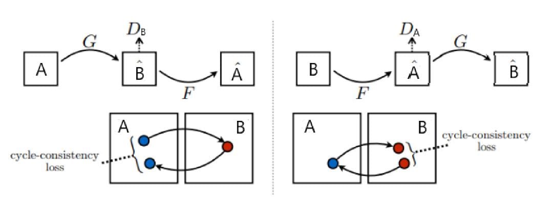
Specifically, image from Domain A undergoes image translation to Domain B via Generator B and then Generator A should be able to take that same generated image and translate it back to Domain A which should bring it back to the original image.
There is one further element to the architecture, referred to as the identity mapping. This is where a generator is provided with images as input from the target domain and is expected to generate the same image without change. This addition to the architecture is optional, although it results in a better matching of the color profile of the input image.
- Domain A -> Generator A -> Domain A
- Domain B -> Generator B -> Domain B
Don’t worry if all of this interplay between the models is still a little fuzzy to you, it’ll start to make more and more sense as getting to the coding example.
Off we go then, to the coding example!
The Problem Statement.
For the coding example of the CycleGAN, we’ll take up an interesting case presented in the research paper, which we’ve also used as one of the examples to explain concepts in this blog- the horse to zebra and zebra to horse unpaired image translation. To state the obvious, in this problem we’ll be converting a horse to a zebra and also be converting zebras to horses using unpaired images.
We’ll be using the same model architecture and configuration described in the CycleGAN paper to facilitate a better correlation between what the readers read in the paper to what they implement for real themselves. The author provides a fully working implementation of the CycleGAN already but written and compiled in the PyTorch Deep Learning Framework. Since for the majority of the blogs here, we’ve preferred the TensorFlow based Keras Deep Learning Framework, we’ll follow implementation in Keras itself and possibly take up PyTorch in the upcoming blogs since PyTorch is steadily gaining popularity along with the more popular Keras.
The Dataset.
The link to the dataset which we’ll be using this section onwards is provided below.
The zip file for this dataset about 111 megabytes and can be downloaded from the CycleGAN webpage:
- Download Horses to Zebras Dataset (111 megabytes)
We will refer to this dataset as “horses2zebra“ . We can refer to this as “zebras2horses’ equivalently since we’ll be performing both the tasks with the same model, but for the purposes of convenience and standardization, we’ve referred to the dataset as “horses2zebra” throughout the blog.
After downloading the dataset into your current working directory.
You will see the following directory structure:
horse2zebra
├── testA
├── testB
├── trainA
└── trainB
The “A” category refers to a horse and “B” category refers to zebra, and the dataset is comprised of the train and test elements. For this blog, we will load all photographs and use them as a training dataset but the readers are free to keep the directories as is.
The images are square with the shape 256×256.
Loading the Dataset.
The first step is always to load all the images from the stored location into the memory so that we can train on them.
The code below will load all images from the train and test folders and create an array of images for category A and another for category B.
Both arrays are then saved to a new file in compressed NumPy array format so that we can use it later anytime instead of going through the entire process again.
# example of preparing the horses and zebra dataset

from os import listdir
from numpy import asarray
from numpy import vstack
from keras.preprocessing.image import img_to_array
from keras.preprocessing.image import load_img
from numpy import savez_compressed


# load all images in a directory into memory

def load_images(path, size=(256,256)):
	data_list = list()
	# enumerate filenames in directory, assume all are images
	for filename in listdir(path):
		# load and resize the image
		pixels = load_img(path + filename, target_size=size)
		# convert to numpy array
		pixels = img_to_array(pixels)
		# store
		data_list.append(pixels)
	return asarray(data_list)

# dataset path
path = 'horse2zebra/'
# load dataset A
dataA1 = load_images(path + 'trainA/')
dataAB = load_images(path + 'testA/')
dataA = vstack((dataA1, dataAB))
print('Loaded dataA: ', dataA.shape)
# load dataset B
dataB1 = load_images(path + 'trainB/')
dataB2 = load_images(path + 'testB/')
dataB = vstack((dataB1, dataB2))
print('Loaded dataB: ', dataB.shape)
# save as compressed numpy array
filename = 'horse2zebra_256.npz'
savez_compressed(filename, dataA, dataB)
print('Saved dataset: ', filename)
Running the example first loads all images into memory, showing that there are 1,187 photos in category A (horses) and 1,474 in category B (zebras).
The arrays are then saved in compressed NumPy format with the filename “horse2zebra_256.npz“. Note: this data file is about 570 megabytes, larger than the raw images as we are storing pixel values as 32-bit floating-point values.
We can then load the dataset and plot some of the photos to confirm that we are handling the image data correctly:
# load and plot the prepared dataset

from numpy import load
from matplotlib import pyplot

# load the dataset

data = load('horse2zebra_256.npz')
dataA, dataB = data['arr_0'], data['arr_1']
print('Loaded: ', dataA.shape, dataB.shape)

# plot source images

n_samples = 3
for i in range(n_samples):
	pyplot.subplot(2, n_samples, 1 + i)
	pyplot.axis('off')
	pyplot.imshow(dataA[i].astype(‘uint8’))

# plot target image

for i in range(n_samples):
	pyplot.subplot(2, n_samples, 1 + n_samples + i)
	pyplot.axis('off')
	pyplot.imshow(dataB[i].astype('uint8'))
pyplot.show()
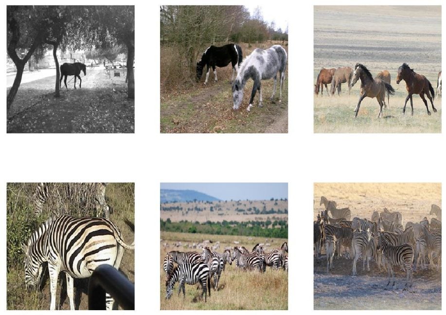
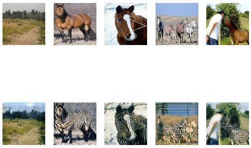
A plot is created showing a row of three images from the horse photo dataset (dataA) and a row of three images from the zebra dataset (dataB).
Notice that each example of horses and zebras is unpaired and that there is no correspondence in orientation, pose, backdrop or surrounding between two pairs at all.
Now that we have prepared the dataset for modeling, we can proceed to develop our CycleGAN.
The Discriminators.
As we know, the discriminator is a Convolutional Neural Network that performs image classification. In our case, it will take an image as input and predict the likelihood of whether that image is a real or fake image. Two discriminator models are used, one for Domain A (horses) and one for Domain B (zebras) as previously stated.
The CycleGAN, like the pix2pix GAN uses the PatchGAN discriminator model configuration.
We’ve already described the PatchGAN in the pix2pix blog, but a quick revision here will be sufficient for the uninformed reader to grasp the concept.
What is the patch-gan?
The discriminator design of the CycleGAN is based on the effective receptive field of the model, which defines the relationship between one output of the model to the number of pixels in the input image. This is called a PatchGAN model and is carefully designed so that each output prediction of the model maps to a 70×70 square or patch of the input image. The benefit of this approach is that the same model can be applied to input images of different sizes, e.g. larger or smaller than 256×256 pixels.
The output of the model depends on the size of the input image but maybe one value or a square activation map of values. Each value is a probability for the likelihood that a patch in the input image is real. These values can be averaged to give an overall likelihood or classification score if needed.
Batch Normalization VS. Instance Normalization Layers
Unlike other models, the CycleGAN discriminator uses InstanceNormalization instead of BatchNormalization.
It is a very simple type of normalization and involves standardizing like scaling to a standard Gaussian, the values on each output feature map, rather than across features in a batch which is done by BatchNormalization.
An implementation of InstanceNormalization is provided in the Keras-contrib project that provides early access to community supplied Keras features.
The Keras-contrib library can be installed via pip as follows:
sudo pip install git+https://www.github.com/keras-team/keras-contrib.git
With that out of the way, let’s now move on to our discriminator models.
First, we’ll define all the necessary imports.
#the necessary imports

from random import random
from numpy import load
from numpy import zeros
from numpy import ones
from numpy import asarray
from numpy.random import randint
from keras.optimizers import Adam
from keras.initializers import RandomNormal
from keras.models import Model
from keras.models import Input
from keras.layers import Conv2D
from keras.layers import Conv2DTranspose
from keras.layers import LeakyReLU
from keras.layers import Activation
from keras.layers import Concatenate
from keras_contrib.layers.normalization.instancenormalization import InstanceNormalization
from matplotlib import pyplot
Next, we’ll define the discriminator model.
The define_discriminator() function below implements the 70×70 PatchGAN discriminator model as per the design of the model in the paper. The model takes a 256×256 sized image as input and outputs a patch of predictions. The model is optimized using least-squares loss (L2) implemented as a mean squared error, and weighting is used so that updates to the model have half (0.5) the usual effect. The authors of CycleGAN paper recommend this weighting of model updates to slow down changes to the discriminator, relative to the generator model during training.
# define the discriminator model

def define_discriminator(image_shape):
	# weight initialization
	init = RandomNormal(stddev=0.02)
	# source image input
	in_image = Input(shape=image_shape)
	# C64
	d = Conv2D(64, (4,4), strides=(2,2), padding='same', kernel_initializer=init)(in_image)
	d = LeakyReLU(alpha=0.2)(d)
	# C128
	d = Conv2D(128, (4,4), strides=(2,2), padding='same', kernel_initializer=init)(d)
	d = InstanceNormalization(axis=-1)(d)
	d = LeakyReLU(alpha=0.2)(d)
	# C256
	d = Conv2D(256, (4,4), strides=(2,2), padding='same', kernel_initializer=init)(d)
	d = InstanceNormalization(axis=-1)(d)
	d = LeakyReLU(alpha=0.2)(d)
	# C512
	d = Conv2D(512, (4,4), strides=(2,2), padding='same', kernel_initializer=init)(d)
	d = InstanceNormalization(axis=-1)(d)
	d = LeakyReLU(alpha=0.2)(d)
	# second last output layer
	d = Conv2D(512, (4,4), padding='same', kernel_initializer=init)(d)
	d = InstanceNormalization(axis=-1)(d)
	d = LeakyReLU(alpha=0.2)(d)
	# patch output
	patch_out = Conv2D(1, (4,4), padding='same', kernel_initializer=init)(d)
	# define model
	model = Model(in_image, patch_out)
	# compile model
	model.compile(loss='mse', optimizer=Adam(lr=0.0002, beta_1=0.5), loss_weights=[0.5])
	return model
The discriminator model architecture is the same for Domains A and B. So just one definition of the architecture will suffice and we can just call the define_discriminator() twice for both Domain A and Domain B during execution which we will see shortly.
That’s it for the discriminator, next up: the generator.
The Generator.
The generator model architecture is rather more complex but at the heart of it is still the encoder-decoder structure we had in the pix2pix GAN generator.
We’ll quickly summarise the encoder-decoder architecture used in the pix2pix GAN for the readers that didn’t have a chance to go through it before explaining the complexities that the CycleGAN generator has added on.
The basic encoder-decoder structure (pix2pix) used was the U-Net Architecture as shown:
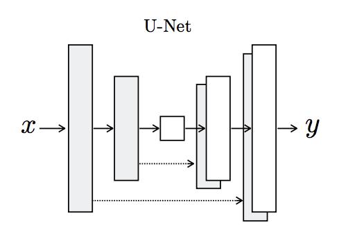
From the schematic, the most basic intuition that can be developed is that the model first downsamples or encodes the input image down to a bottleneck layer, then upsamples or decodes the bottleneck representation to the size of the output image.
But that doesn’t explain the dotted arrows going from the downsampling layers to the upsampling layers. These dotted arrows are called ‘skip connections’ which concatenates the output of the downsampling convolution layers with the feature maps from the upsampling convolution layers at the same level. By the same level, we mean, the same dimension. To be even more concrete, the skip connection from a downsampling layer that has output dimensions, say, 128x128x256 will be concatenated with an upsampling layer that has output dimensions of 128x128x256. Since the network is symmetric, every downsampling layer will have a corresponding upsampling counterpart to facilitate skip connections between.
This was the pix2pix GAN generator configuration.
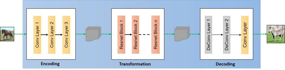
The CycleGAN generator is the same in that it also an encoder-decoder model architecture that takes a source image (e.g. horse image) and generates a target image (e.g. zebra image) by downsampling or encoding the input image down to a bottleneck layer. But it is different than the pix2pix generator in that the encodings are interpreted with a number of ResNet layers that use skip connections, followed by a series of layers that upsample or decode the representation to the size of the output image which again, follows the pix2pix generator scheme.
Below is a schematic representation of the CycleGAN generator:
What are these resnet blocks?
As daunting it may sound, the concept is actually pretty simple and something the reader is actually familiar with already.
In traditional neural networks, each layer feeds into the next layer. In a network with residual blocks, each layer feeds into the next layer and directly into the layers about 2–3 hops away. That’s it.
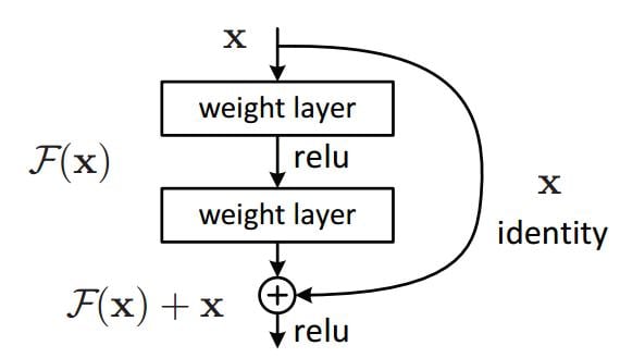
As can be seen from the image, some layers are being ‘skipped’ over. In the pix2pix generator model, we use skip connections going from the downsampled to upsampled layers. Whereas in the CycleGAN, we use skip connections within the downsampling layers after the bottleneck layer and not going from the downsampled layers to the upsampled layers.
The code for the generator will help make this clear:
First, we need a function to define the ResNet blocks. These are blocks comprised of two 3×3 Convolutional layers where the input to the block is concatenated to the output of the block, channel-wise.
# generator a resnet block

def resnet_block(n_filters, input_layer):
	# weight initialization
	init = RandomNormal(stddev=0.02)
	# first layer convolutional layer
	g = Conv2D(n_filters, (3,3), padding='same', kernel_initializer=init)(input_layer)
	g = InstanceNormalization(axis=-1)(g)
	g = Activation('relu')(g)
	# second convolutional layer
	g = Conv2D(n_filters, (3,3), padding='same', kernel_initializer=init)(g)
	g = InstanceNormalization(axis=-1)(g)
	# concatenate merge channel-wise with input layer
	g = Concatenate()([g, input_layer])
	return g
Next, we can define a function that will create the 9-resnet block version for 256×256 input images.
# define the generator model

def define_generator(image_shape, n_resnet=9):
	# weight initialization
	init = RandomNormal(stddev=0.02)
	# image input
	in_image = Input(shape=image_shape)

	g = Conv2D(64, (7,7), padding='same', kernel_initializer=init)(in_image)
	g = InstanceNormalization(axis=-1)(g)
	g = Activation('relu')(g)
	# d128
	g = Conv2D(128, (3,3), strides=(2,2), padding='same', kernel_initializer=init)(g)
	g = InstanceNormalization(axis=-1)(g)
	g = Activation('relu')(g)
	# d256
	g = Conv2D(256, (3,3), strides=(2,2), padding='same', kernel_initializer=init)(g)
	g = InstanceNormalization(axis=-1)(g)
	g = Activation('relu')(g)
	# R256
	for _ in range(n_resnet):
		g = resnet_block(256, g)
	# u128
	g = Conv2DTranspose(128, (3,3), strides=(2,2), padding='same', kernel_initializer=init)(g)
	g = InstanceNormalization(axis=-1)(g)
	g = Activation('relu')(g)
	# u64
	g = Conv2DTranspose(64, (3,3), strides=(2,2), padding='same', kernel_initializer=init)(g)
	g = InstanceNormalization(axis=-1)(g)
	g = Activation('relu')(g)

	g = Conv2D(3, (7,7), padding='same', kernel_initializer=init)(g)
	g = InstanceNormalization(axis=-1)(g)
	out_image = Activation('tanh')(g)
	# define model
	model = Model(in_image, out_image)
	return model
Just like the discriminator, the generator models for both the Domains A and B have the same configuration so we will just call this function twice during execution as we’ll shortly see.
Let’s tie all the models up together and define our CycleGAN!
The GAN.
Before we can actually talk about the composite model, we need to talk about the losses.
Losses.
We know that the discriminator models are directly trained on images whereas the generator models are updated to minimize the loss predicted by the discriminator for generated images marked as “real“, called adversarial loss. As such, they are encouraged to generate images that better fit into the target domain.
The generator models are also updated based on how effective they are at the regeneration of a source image when used with the other generator model, called cycle loss. Finally, a generator model is expected to output an image without translation when provided an example from the target domain, called identity loss.
Altogether, each generator model is optimized via the combination of four outputs with four-loss functions:
- Adversarial loss (L2 or mean squared error).
- Identity loss (L1 or mean absolute error).
- Forward cycle loss (L1 or mean absolute error).
- Backward cycle loss (L1 or mean absolute error).
This is implemented in the define_composite_model() function below that takes a defined generator model (g_model_1) as well as the defined discriminator model for the generator models output (d_model) and the other generator model (g_model_2).
The discriminator is connected to the output of the generator in order to classify generated images as real or fake. A second input for the composite model is defined as an image from the target domain (instead of the source domain), which the generator is expected to output without translation for the identity mapping. Next, forward cycle loss involves connecting the output of the generator to the other generator, which will reconstruct the source image. Finally, the backward cycle loss involves the image from the target domain used for the identity mapping that is also passed through the other generator whose output is connected to our main generator as input and outputs a reconstructed version of that image from the target domain.
To summarise, a composite model has two inputs for the real photos from Domain A and Domain B, and four outputs for the discriminator output, identity generated image, forward cycle generated an image, and backward cycle generated image.
# define a composite model

def define_composite_model(g_model_1, d_model, g_model_2, image_shape):
	# ensure the model we're updating is trainable
	g_model_1.trainable = True
	# mark discriminator as not trainable
	d_model.trainable = False
	# mark other generator model as not trainable
	g_model_2.trainable = False
	# discriminator element
	input_gen = Input(shape=image_shape)
	gen1_out = g_model_1(input_gen)
	output_d = d_model(gen1_out)
	# identity element
	input_id = Input(shape=image_shape)
	output_id = g_model_1(input_id)
	# forward cycle
	output_f = g_model_2(gen1_out)
	# backward cycle
	gen2_out = g_model_2(input_id)
	output_b = g_model_1(gen2_out)
	# define model graph
	model = Model([input_gen, input_id], [output_d, output_id, output_f, output_b])
	# define optimization algorithm configuration
	opt = Adam(lr=0.0002, beta_1=0.5)
	# compile model with weighting of least squares loss and L1 loss
	model.compile(loss=['mse', 'mae', 'mae', 'mae'], loss_weights=[1, 5, 10, 10], optimizer=opt)
	return model
We need to create a composite model for each generator model, e.g. the Generator A (B to A) for zebra to horse translation, and the Generator B (A to B) for horse to zebra translation.
We understand all of this gets confusing for the reader, but there’s nothing like a good summary that can help etch the concept in your minds. Keeping that in mind, we’ve prepared a table that explains how each image moves in the models and how each loss is calculated.
Generator A Composite Model (B to A or Zebra to Horse)
The inputs, transformations, and outputs of the model are as follows:
| Loss | From | Via | To | Via | To | Loss Calculated Between |
| Adversarial Loss | Domain B | Generator A | Domain A | – | – | Generated Domain A Image & Discriminator for Domain A |
| Identity Loss | Domain A | Generator A | Domain A | – | – | Original Domain A Image & Generated Domain A Image |
| Forward Cycle Loss | Domain B | Generator A | Domain A | Generator B | Domain B | Original Domain B Image and Reconstructed Domain B Image |
| Backward Cycle Loss | Domain A | Generator B | Domain B | Generator B | Domain A | Original Domain A Image and Reconstructed Domain A Image |
Generator B Composite Model (A to B or Horse to Zebra)
The inputs, transformations, and outputs of the model are as follows:
| Loss | From | Via | To | Via | To | Loss Calculated Between |
| Adversarial Loss | Domain A | Generator B | Domain B | – | – | Generated Domain B Image & Discriminator for Domain B |
| Identity Loss | Domain B | Generator B | Domain B | – | – | Original Domain B Image & Generated Domain B Image |
| Forward Cycle Loss | Domain A | Generator B | Domain B | Generator A | Domain A | Original Domain A Image and Reconstructed Domain A Image |
| Backward Cycle Loss | Domain B | Generator A | Domain A | Generator B | Domain B | Original Domain B Image and Reconstructed Domain B Image |
Defining the models is the hard part of the CycleGAN; the rest is standard GAN training and relatively straightforward which most of the readers must be familiar with by now.
Training.
Next, we can load our paired images dataset in compressed NumPy array format. This will return a list of two NumPy arrays: the first for source images and the second for corresponding target images.
# load and prepare training images

def load_real_samples(filename):
	# load the dataset
	data = load(filename)
	# unpack arrays
	X1, X2 = data['arr_0'], data['arr_1']
	# scale from [0,255] to [-1,1]
	X1 = (X1 - 127.5) / 127.5
	X2 = (X2 - 127.5) / 127.5
	return [X1, X2]
Each training iteration we will require a sample of real images from each domain as input to the discriminator and composite generator models. This can be achieved by selecting a random batch of samples.
The generate_real_samples() function below implements this


# select a batch of random samples, returns images and target

def generate_real_samples(dataset, n_samples, patch_shape):
	# choose random instances
	ix = randint(0, dataset.shape[0], n_samples)
	# retrieve selected images
	X = dataset[ix]
	# generate 'real' class labels (1)
	y = ones((n_samples, patch_shape, patch_shape, 1))
	return X, y
Similarly, a sample of generated images is required to update each discriminator model in each training iteration.
The generate_fake_samples() function below generates this sample given a generator model and the sample of real images from the source domain.
# generate a batch of images, returns images and targets

def generate_fake_samples(g_model, dataset, patch_shape):
	# generate fake instance
	X = g_model.predict(dataset)
	# create 'fake' class labels (0)
	y = zeros((len(X), patch_shape, patch_shape, 1))
	return X, y
Since we are to strictly follow the implementation described in the paper, we will define an image pool of 50 generated images for each discriminator model that is first populated and probabilistically either adds new images to the pool by replacing an existing image or uses a generated image directly. We can implement this as a Python list of images for each discriminator and use the update_image_pool() function below to maintain each pool list.
# update image pool for fake images

def update_image_pool(pool, images, max_size=50):
	selected = list()
	for image in images:
		if len(pool) < max_size:
			# stock the pool
			pool.append(image)
			selected.append(image)
		elif random() < 0.5:
			# use image, but don't add it to the pool
			selected.append(image)
		else:
			# replace an existing image and use replaced image
			ix = randint(0, len(pool))
			selected.append(pool[ix])
			pool[ix] = image
	return asarray(selected)
We can now define the training of each of the generator models.
The train() function below takes all six models (two discriminator, two generator, and two composite models) as arguments along with the dataset and trains the models.
# train the cycleGAN model

def train(d_model_A, d_model_B, g_model_AtoB, g_model_BtoA, c_model_AtoB, c_model_BtoA, dataset):

	# define properties of the training run
	n_epochs, n_batch, = 100, 1
	# determine the output square shape of the discriminator
	n_patch = d_model_A.output_shape[1]
	# unpack dataset
	trainA, trainB = dataset
	# prepare image pool for fakes
	poolA, poolB = list(), list()
	# calculate the number of batches per training epoch
	bat_per_epo = int(len(trainA) / n_batch)
	# calculate the number of training iterations
	n_steps = bat_per_epo * n_epochs
	# manually enumerate epochs
	for i in range(n_steps):
		# select a batch of real samples
		X_realA, y_realA = generate_real_samples(trainA, n_batch, n_patch)
		X_realB, y_realB = generate_real_samples(trainB, n_batch, n_patch)
		# generate a batch of fake samples
		X_fakeA, y_fakeA = generate_fake_samples(g_model_BtoA, X_realB, n_patch)
		X_fakeB, y_fakeB = generate_fake_samples(g_model_AtoB, X_realA, n_patch)
		# update fakes from pool
		X_fakeA = update_image_pool(poolA, X_fakeA)
		X_fakeB = update_image_pool(poolB, X_fakeB)
		# update generator B->A via adversarial and cycle loss
		g_loss2, _, _, _, _  = c_model_BtoA.train_on_batch([X_realB, X_realA], [y_realA, X_realA, X_realB, X_realA])
		# update discriminator for A -> [real/fake]
		dA_loss1 = d_model_A.train_on_batch(X_realA, y_realA)
		dA_loss2 = d_model_A.train_on_batch(X_fakeA, y_fakeA)
		# update generator A->B via adversarial and cycle loss
		g_loss1, _, _, _, _ = c_model_AtoB.train_on_batch([X_realA, X_realB], [y_realB, X_realB, X_realA, X_realB])
		# update discriminator for B -> [real/fake]
		dB_loss1 = d_model_B.train_on_batch(X_realB, y_realB)
		dB_loss2 = d_model_B.train_on_batch(X_fakeB, y_fakeB)
		# summarize performance
		print('>%d, dA[%.3f,%.3f] dB[%.3f,%.3f] g[%.3f,%.3f]' % (i+1, dA_loss1,dA_loss2, dB_loss1,dB_loss2, g_loss1,g_loss2))
		# evaluate the model performance every so often
		if (i+1) % (bat_per_epo * 1) == 0:
			# plot A->B translation
			summarize_performance(i, g_model_AtoB, trainA, 'AtoB')
			# plot B->A translation
			summarize_performance(i, g_model_BtoA, trainB, 'BtoA')
		if (i+1) % (bat_per_epo * 5) == 0:
			# save the models
			save_models(i, g_model_AtoB, g_model_BtoA)
The example can be run on CPU hardware, although GPU hardware is recommended because this example might take a number of hours to run even on modern GPU hardware so we highly recommended using GPU hardware such as the ones provided on Kaggle.
Evaluation.
Into the third GAN blog, we know that GAN models do not typically converge; instead, an equilibrium is found between the generator and discriminator models. As such, we cannot easily judge whether training should stop. Therefore, we can save the model and use it to generate sample image-to-image translations periodically during training, such as every one or five training epochs.
We can then review the generated images at the end of training and use the image quality to choose a final model.
The save_models() and the summarize_performance() functions below will save each generator model to the current directory along with a plot of randomly selected images from that particular model.
# save the generator models to file

def save_models(step, g_model_AtoB, g_model_BtoA):
	# save the first generator model
	filename1 = 'g_model_AtoB_%06d.h5' % (step+1)
	g_model_AtoB.save(filename1)
	# save the second generator model
	filename2 = 'g_model_BtoA_%06d.h5' % (step+1)
	g_model_BtoA.save(filename2)
	print('>Saved: %s and %s' % (filename1, filename2))

# generate samples and save as a plot and save the model

def summarize_performance(step, g_model, trainX, name, n_samples=5):
	# select a sample of input images
	X_in, _ = generate_real_samples(trainX, n_samples, 0)
	# generate translated images
	X_out, _ = generate_fake_samples(g_model, X_in, 0)
	# scale all pixels from [-1,1] to [0,1]
	X_in = (X_in + 1) / 2.0
	X_out = (X_out + 1) / 2.0
	# plot real images
	for i in range(n_samples):
		pyplot.subplot(2, n_samples, 1 + i)
		pyplot.axis('off')
		pyplot.imshow(X_in[i])
	# plot translated image
	for i in range(n_samples):
		pyplot.subplot(2, n_samples, 1 + n_samples + i)
		pyplot.axis('off')
		pyplot.imshow(X_out[i])
	# save plot to file
	filename1 = '%s_generated_plot_%06d.png' % (name, (step+1))
	pyplot.savefig(filename1)
	pyplot.close()
The plots of generated images can be used to choose a model and more training iterations may not necessarily mean better quality generated images.
Horses to Zebras translation starts to become reliable after about 50 epochs.
The translation from Zebras to Horses appears to be more challenging for the model to learn, although somewhat plausible translations also begin to be generated after 50 to 60 epochs.
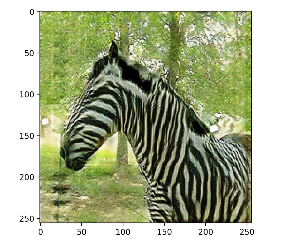
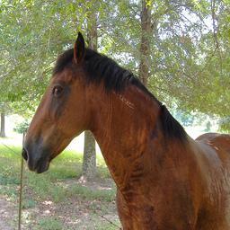
After you’ve selected an optimum model, you can actually test out the CycleGAN by using images that are from the dataset or even outside the dataset. We’ve tried one image and it looks as if CycleGAN came through for us.
Whew! That was a long ride. We hope the reader has had as much fun understanding and coding as much as we did curate it.
We promised the readers something big in the previous, we hope this blog has lived up to all your expectations.
In the adventure spanning 4 blogs, covering three types of GANs, we’ve seen the prowess of GANs and justified why they caused such disruption when they arrived in 2014 in a paper by Ian Goodfellow and company.
We started this series with Yann LeCun’s famous quote on GANs,
“The most interesting idea in deep learning in the last 20 years.”
And standing at this GAN series’ penultimate stage, we do hope we’ve done our bit in helping the readers understand why.
But we’re not done.
In these 4 blogs, we focused on the concepts and code which left us little room to explore the variety of applications of GANs in the world today. So accordingly, in the last and final blog of this series, we’ll bring to you all the applications where GANs are used today in full color and thoroughly dissect each of them with you, the pros, as well as the cons.
We understand this blog has been a bit heavy on our readers and the reader might still be a little ambiguous about the entire CycleGAN process, but we’d like to tell y’all that that’s completely okay. CycleGANs are incredibly difficult to grasp in one go and it’s alright to go over this blog twice or even thrice because, at the end of the day, incomplete knowledge is more dangerous than no knowledge.
And as compensation for this blog in terms of heaviness, we promise a fun-filled, adventurous blog to properly wrap up this GAN series on a high note.
As always, all your doubts and comments are welcome in the comments section. If you’d like us to cover more variants of GANs, do let us know.
Lastly, we leave you with this link to the official CycleGAN project on GitHub which has loads of examples like GTA landscape to real landscape translations among other interesting use cases for the reader to marvel at!
https://junyanz.github.io/CycleGAN/
Have a good day! And do tune in for the next blog!
Other Blogs from GAN Series
- An Introduction to Generative Adversarial Networks- Part 1
- Introduction to Generative Adversarial Networks with Code- Part 2
- pix2pix GAN: Bleeding Edge in AI for Computer Vision- Part 3
- The Grand Finale: Applications of GANs- Part 5
Read More:
- Artificial Intelligence in Space Exploration
- AI Dueling: Witness the New Frontier of Artificial Intelligence
- Artificial Intelligence Vs Business Intelligence
- Role of Artificial Intelligence In Google Android 9.0 Pie
- How Smart Contract can Make our Life Better?
- Why Every Business Should Use Machine Learning?
Looking for Online Learning? Here’s what you can choose from!
- Deep Learning & Neural Networks Using Python & Keras For Dummies
- Learn Machine Learning By Building Projects
- Machine Learning With TensorFlow The Practical Guide
- Deep Learning & Neural Networks Python Keras For Dummies
- Mathematical Foundation For Machine Learning and AI
References
- Unpaired Image-to-Image Translation using Cycle-Consistent Adversarial Networks by Jun-Yan Zhu, Taesung Park, Phillip Isola, Alexei A. Efros
- Image-to-Image Translation with Conditional Adversarial Networks Phillip Isola, Jun-Yan Zhu, Tinghui Zhou, Alexei A. Efros
- Generative Adversarial Networks Ian J. Goodfellow, Jean Pouget-Abadie, Mehdi Mirza, Bing Xu, David Warde-Farley, Sherjil Ozair, Aaron Courville, Yoshua Bengio
- https://people.eecs.berkeley.edu/~taesung_park/CycleGAN/datasets/
- https://machinelearningmastery.com/cyclegan-tutorial-with-keras/
- https://hardikbansal.github.io/CycleGANBlog/
- https://github.com/junyanz/pytorch-CycleGAN-and-pix2pix