

“Hello and a warm welcome to this blog where all the action is about to happen!
Two Neural Networks are going to face off each other and only one of them will be left standing!
The only question is, which one are you rooting for?
The Generator or the Discriminator?
We’re sorry if we’re hyping up this thing a little.

Okay fine, we’re totally overdoing it.
But we promise you’ll share our enthusiasm too by the end of this blog.
Before we begin, for the readers that have stumbled upon this blog first, we’d like you all to know that we’ve done a conceptual introduction of GANs in our previous blog, Introduction to Generative Adversarial Networks- Part 1. We highly recommend you to go through that blog because the code in this one requires you to have a thorough conceptual understanding of the entire idea behind GANs which we’ve covered with a jargon-free analogy. It neither assumes nor requires any advanced previous AI knowledge. That’s the way we always keep it at Eduonix.
Right then.
It’s about time.
GANs IN ACTION!
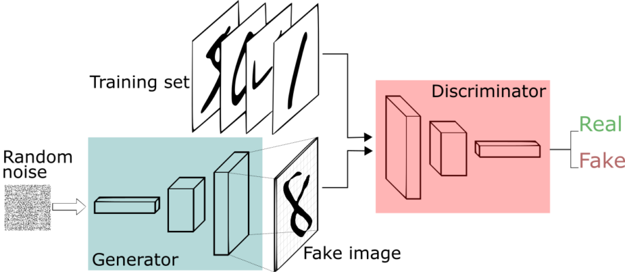
So the problem statement we have to generate handwritten digits like those found in the MNIST dataset.
Here, the goal of our discriminator, when shown an instance from the true MNIST dataset, would be to recognize those that are authentic.
Meanwhile, our generator is creating new, synthetic images that it passes to the discriminator. This would be you with the canvas trying to replicate the painting in our analogy. The generator does this in the hopes that the generated images, too, will be deemed authentic by the discriminator (our art expert), even though they are fake. The goal of the generator is to generate plausible handwritten digits, which is to lie without being caught. The goal of the discriminator is to identify images coming from the generator as fake.
In Situation B, your first attempt at the painting wouldn’t be too accurate. In fact, it would hardly represent anything like the original painting. The analogy for this in GANs is that we start out the generator by passing it random noise which eventually learns to mold into plausible handwritten digits images.
We illustrate the scenario below:
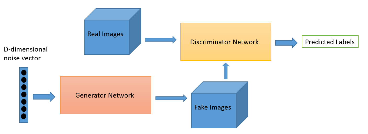
For our use case, the discriminator network is a standard convolutional network that can categorize the images fed to it, a binomial classifier labeling images as real or fake. The generator is an inverse convolutional network, in the sense that while a standard convolutional classifier takes an image and downsamples it to produce a probability, the generator takes a vector of random noise and upsamples it to an image. The first throws away data through downsampling techniques like MaxPooling, and the second generates new data.
Both nets are trying to optimize a different and opposing objective function, or loss function.
This is essentially our student and art expert model. As the discriminator changes it’s behavior, looking for more and more finer details of the image produced, so does the generator by generating more and more plausible images and vice versa. Their losses push against each other.
Now that the groundwork is laid, we’ll move on to some code. But before that, here’s the final structure of the GAN that we’ll be training:
Right! Let’s move on to some code then.
I. Importing Libraries
import numpy as np
import pandas as pd
import keras
from keras.layers import Conv2D, Conv2DTranspose, Dropout, Input, Flatten, LeakyReLU, Dense
from keras.models import Model, Sequential
from keras.datasets import mnist
from keras.layers.advanced_activations import LeakyReLU
from keras.optimizers import adam
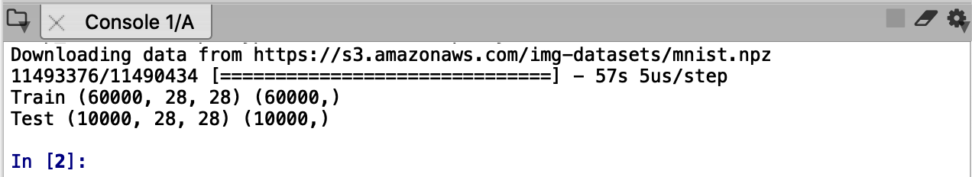
II. Loading the MNIST Dataset
# load the images into memory
(trainX, trainy), (testX, testy) = mnist.load_data()
# summarize the shape of the dataset
print('Train', trainX.shape, trainy.shape)
print('Test', testX.shape, testy.shape)
Running the above code will result in the following output:
In case, the readers are unaware of the MNIST dataset, we recommend you check out our earlier blogs out on the Deep Learning with Keras Series where we take up several Neural Network architectures and try to solve various problems using Deep Learning.
Read More:
- Deep Neural Networks with Keras
- Functional API of Keras
- Convolutional Neural Networks with Keras
- Recurrent Neural Networks and LSTMs with Keras
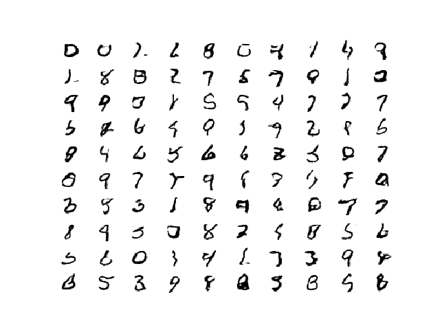
For completeness of this blog, however, we show the MNIST dataset below:
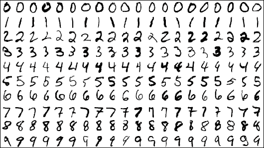
We will use the images in the training dataset as the basis for training a Generative Adversarial Network.
Specifically, the generator model will learn how to generate new plausible handwritten digits between 0 and 9, using a discriminator that will try to distinguish between real images from the MNIST training dataset and new images output by the generator model.
III. Defining the Discriminator
The role of the discriminator should be now clear to our reader. The discriminator model must take a sample image from our MNIST dataset as input and output a classification prediction as to whether the sample is real or fake.
This is thus, a binary classification problem with input as a 28×28 image and output as the likelihood of whether the sample is real or fake.
As described above, we’ll be using a Convolutional Neural Network for our discriminator. The objective function (or the loss) that’ll aim to minimize will be binary_cross_entropy function appropriate for binary classifications. The choice of our optimizer, by default, will be Adam.
We’ve covered some best practices when defining various Neural Network architectures to model various problems in a blog compiled just for you in the Deeper with Deep Neural Networks, be sure to check it out.
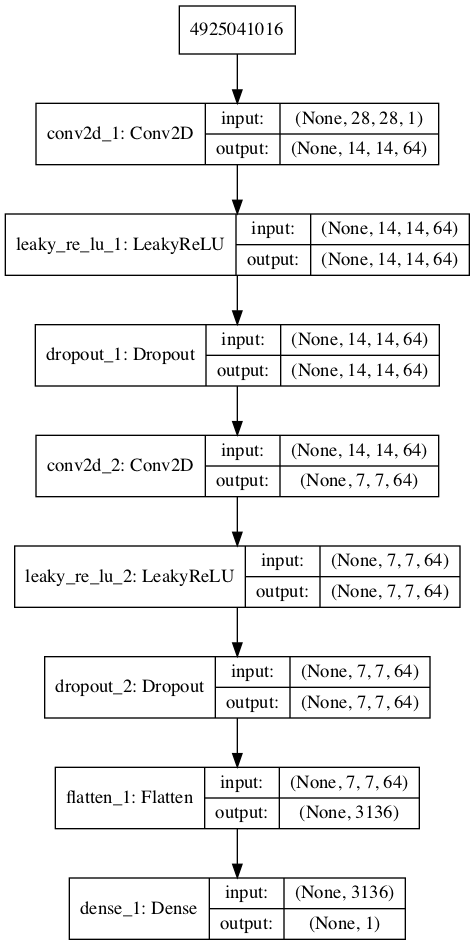
The function define_discriminator() below defines the discriminator model:
def define_discriminator(in_shape=(28,28,1)):
	model = Sequential()
	model.add(Conv2D(64, (3,3), strides=(2, 2), padding='same', input_shape=in_shape))
	model.add(LeakyReLU(alpha=0.2))
	model.add(Dropout(0.4))
	model.add(Conv2D(64, (3,3), strides=(2, 2), padding='same'))
	model.add(LeakyReLU(alpha=0.2))
	model.add(Dropout(0.4))
	model.add(Flatten())
	model.add(Dense(1, activation='sigmoid'))
	# compile model
	opt = Adam(lr=0.0002, beta_1=0.5)
	model.compile(loss='binary_crossentropy', optimizer=opt, metrics=['accuracy'])
	return model
To call define the model now, all we have to do is call the define_discriminator() function in our code. We always recommend to print out the summary of the model you’ve created as a good practice along with the plot of the model so that it’s easy for you to spot any error you might have made during model definition.
# define model
model = define_discriminator()
# summarize the model
model.summary()
# plot the model
plot_model(model, to_file='discriminator_plot.png', show_shapes=True, show_layer_names=True)
The plot of the model that we expect is shown below:
If you reckon, the discriminator has to discriminate the real images from the fake ones. Currently, all we have are the real images that are in the trainX variable. We do not have any fake images. So we’ll have to go about sorting that part out.
First, we’ll need to load and prepare the dataset of real images and then we’ll worry about the fake samples.
It should be noted that the images are 2D arrays of pixels and Convolutional Neural Networks expect 3D arrays of images as input, where each image has one or more channels.
Consequently, we must update the images to have an additional dimension for the grayscale channel. We can do this using the expand_dims() function provided by NumPy and specify the final dimension for the channels-last image format.
def load_real_samples():
	# expand to 3d, e.g. add channels dimension
	X = expand_dims(trainX, axis=-1)
	# convert from unsigned ints to floats
	X = X.astype('float32')
	# scale from [0,255] to [0,1]
	X = X / 255.0
	return X
Now for training, the model will be updated in batches, specifically with a collection of real samples and a collection of generated samples.
So we write another function called the generate_real_samples() function below which will take the training dataset as an argument and will select a random subsample of images; it will also return class labels for the sample, specifically a class label of 1, to indicate real images.
def generate_real_samples(dataset, n_samples):
	# choose random instances
	ix = randint(0, dataset.shape[0], n_samples)
	# retrieve selected images
	X = dataset[ix]
	# generate 'real' class labels (1)
	y = ones((n_samples, 1))
	return X, y
There. We’ve sorted out the real samples. Now for the fake samples.
We don’t have a generator model yet, so instead, we can generate images comprised of random pixel values, specifically random pixel values in the range [0,1] like our scaled real images. We’ve defined the generate_fake_samples() function below to generate fake images.
def generate_fake_samples(n_samples):
	# generate uniform random numbers in [0,1]
	X = rand(28 * 28 * n_samples)
	# reshape into a batch of grayscale images
	X = X.reshape((n_samples, 28, 28, 1))
	# generate 'fake' class labels (0)
	y = zeros((n_samples, 1))
	return X, y
Now, we’ll need to train our Discriminative Model.
IV. Training the Discriminative Model.
# train the discriminator model
def train_discriminator(model, dataset, n_iter=100, n_batch=256):
half_batch = int(n_batch / 2)
# manually enumerate epochs
for i in range(n_iter):
# get randomly selected 'real' samples
X_real, y_real = generate_real_samples(dataset, half_batch)
# update discriminator on real samples
_, real_acc = model.train_on_batch(X_real, y_real)
# generate 'fake' examples
X_fake, y_fake = generate_fake_samples(half_batch)
# update discriminator on fake samples
_, fake_acc = model.train_on_batch(X_fake, y_fake)
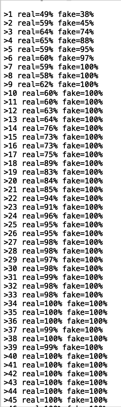
# summarize performance
print('>%d real=%.0f%% fake=%.0f%%' % (i+1, real_acc*100, fake_acc*100))
# define the discriminator model
model = define_discriminator()
# load image data
dataset = load_real_samples()
# fit the model
train_discriminator(model, dataset)
Even though the function might look complicated to you. Here’s what it’s essentially doing, we are using a batch size of 256 images where 128 are real and 128 are fake each iteration. We then update the discriminator separately for real and fake examples so that we can calculate the accuracy of the model on each sample prior to the update. This gives insight into how the discriminator model is performing over time.
You’ll see that in about 40 iterations, it attains peak performance, easily being able to differentiate between fake and the real samples.
Now that we know how to define and train the discriminator model, we need to look at developing the generator model.
V. Defining the Generator
The next step is defining the generator. The generator will start out by outputting random noise at first, analogous to your first crude replication of the painting, and will then eventually learn to mold the randomness into seemingly plausible handwritten digits to pass the discriminator, analogous to your final attempts at getting the painting right to the details.
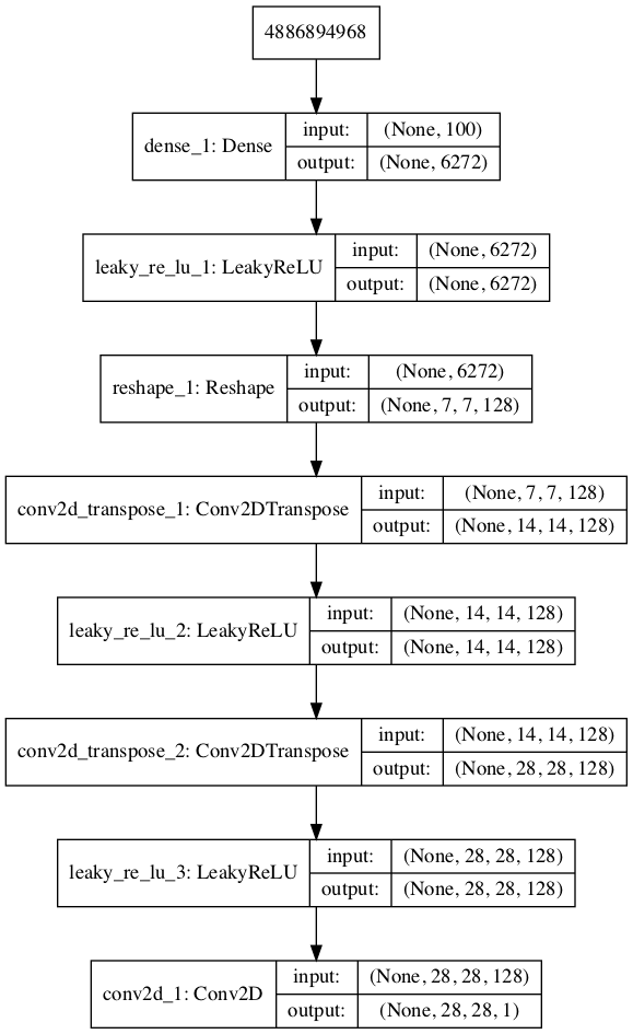
The question here is perhaps, how do we go from random noise to a plausible image? The idea is simple. Like in the case of the discriminator network where we downsampled the image dimensions to obtain a feature map with which the network took the decision of the likelihood of fakeness and realness, in the generator, we go the other way around: That is, we start with something small, and then upsample the image dimensions to give the network space to invent and create. This is achieved by transposed convolutions.
#define the generator model
def define_generator(latent_dim):
	model = Sequential()
	n_nodes = 128 * 7 * 7
	model.add(Dense(n_nodes, input_dim=latent_dim))
	model.add(LeakyReLU(alpha=0.2))
	model.add(Reshape((7, 7, 128)))
	# upsample to 14x14
	model.add(Conv2DTranspose(128, (4,4), strides=(2,2), padding='same'))
	model.add(LeakyReLU(alpha=0.2))
	# upsample to 28x28
	model.add(Conv2DTranspose(128, (4,4), strides=(2,2), padding='same'))
	model.add(LeakyReLU(alpha=0.2))
	model.add(Conv2D(1, (7,7), activation='sigmoid', padding='same'))
	return model

# define the size of the latent space
latent_dim = 100
# define the generator model
model = define_generator(latent_dim)
# summarise the model
model.summary()
# plot the model
plot_model(model, to_file='generator_plot.png', show_shapes=True, show_layer_names=True)
We’ve included the code to summarise and plot the model just for the reader’s convenience and we highly recommend checking the plots and the summary out.
The plot of the generator model is obtained below:
An explanation is in order for the variable, “latent_dim”.
This variable represents the colors and brushes available to you drawing a parallel between GANs and our concept explanation (Situation B). It’s only using these colors and brushes that you’ll be able to draw your painting. Of course, how you learn to use the brushes and the colors, is on you.
This is exactly the case here. That variable represents a distribution of points that the generator can draw from while attempting to generate plausible images. This distribution is essentially random and is also called the latent space or the latent dimension.
We’ll now show you a convenient function to generate this latent dimension or rather, points from the latest dimension.
# generate points in latent space as input for the generator
def generate_latent_points(latent_dim, n_samples):
	# generate points in the latent space
	x_input = randn(latent_dim * n_samples)
	# reshape into a batch of inputs for the network
	x_input = x_input.reshape(n_samples, latent_dim)
	return x_input
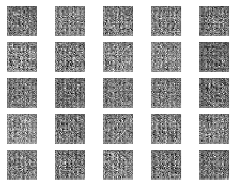
As a matter of fact, this model cannot do much at the moment. We can give it some latent points with which it can generate an image but this image will not nearly represent a handwritten digit since we’ve not oriented the generator towards the handwritten digit generation task.
A question that a reader may ask nevertheless is what happens when we give the latent input to the generator just for the sake of it? What does it ‘generate’?
We’ve shown you exactly what the model would generate.
As expected, the output is essentially random and does not represent a handwritten digit image. This is of course because we haven’t really ‘trained’ the generator to output plausible images.
We’ll use a function from the previous discriminator section to demonstrate the output of the generator to you.
All we have to do is call the predict() method on our model and give it
def generate_fake_samples(g_model, latent_dim, n_samples):
	# generate points in latent space
	x_input = generate_latent_points(latent_dim, n_samples)
	# predict outputs
	X = g_model.predict(x_input)
	# create 'fake' class labels (0) since the images generated are obviously fake
	y = zeros((n_samples, 1))
	return X, y
Now, of course, we want to orient the generator towards generating plausible images which we’ll achieve by training it. It is described in the subsequent section.
VI. Training the Generator Model
Think about Situation B in which you are, essentially, the generator model. How does the process look like?
Let’s go step by step.
- You first output some really off drawings.
- You show the paintings for the expert for his opinion.
- The expert rejects the paintings.
- You go back trying to generate better painting in the hopes to satisfy the expert.
Now let’s take this exact same concept and apply it into GANs.
We have two models now, the generator and the discriminator.
The generator will take input as latent points and generate some image, which the discriminator should asses as fake or real. And based on this feedback by the discriminator, the generator should do better the next time.
So what we’re basically doing is we’re stacking the generator and discriminator such that the generator receives as input random points in the latent space and generates samples that are fed into the discriminator model directly, classified, and the output of this larger model can be used to update the model weights of the generator.
This, dear readers, is the Generative Adversarial Network.
One important note
When training the generator via this GAN model, there are two important changes.
First, we do not change the weights of the discriminator. Since discriminator has already been trained on.
Secondly, we want the discriminator to think that the samples outputted by the generator are real, and not fake.
Now, why would we want to do this? If the discriminator thinks the samples are real from the start, what’s the point?
The answer is simple.
Let us imagine the generator generated a random gibberish image like in the case of the untrained generator model. Now we mark this deliberately as a real sample.
We can imagine that the discriminator will then classify the generated sample as not real (class 0) or a low probability of being real (0.2 or 0.3) since the discriminator is already trained to detect fake and real samples and our inputted image is surely fake.
Now the backpropagation process used to update the model weights will see this as a large error and will update the model weights (i.e. only the weights in the generator since the discriminator weights are fixed) to correct for this error, in turn making the generator better at generating good fake samples.
Therefore, when the generator is trained as part of the GAN model, we will mark the generated samples as real (class 1).
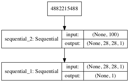
We’ll now define our GAN in accordance with the discussion above:
def define_gan(g_model, d_model):
	# make weights in the discriminator not trainable
	d_model.trainable = False
	model = Sequential()
	# add generator
	model.add(g_model)
	# add the discriminator
	model.add(d_model)
	# compile model
	opt = Adam(lr=0.0002, beta_1=0.5)
	model.compile(loss='binary_crossentropy', optimizer=opt)
	return model

# create the gan
gan_model = define_gan(g_model, d_model)
# summarize gan model
gan_model.summary()
# plot gan model
plot_model(gan_model, to_file='gan_plot.png', show_shapes=True, show_layer_names=True)
The plot of our GAN is shown below:
For GAN training, we’ve defined a function to proceed in the fashion as discussed. We’ve included all the comments necessary for the reader to really understand what is happening with each line.
This concludes the training part of our GAN.
def train(g_model, d_model, gan_model, dataset, latent_dim, n_epochs=100, n_batch=256):
bat_per_epo = int(dataset.shape[0] / n_batch)
half_batch = int(n_batch / 2)
# manually enumerate epochs
for i in range(n_epochs):
# enumerate batches over the training set
for j in range(bat_per_epo):
# get randomly selected 'real' samples
X_real, y_real = generate_real_samples(dataset, half_batch)
# generate 'fake' examples
X_fake, y_fake = generate_fake_samples(g_model, latent_dim, half_batch)
# create training set for the discriminator
X, y = vstack((X_real, X_fake)), vstack((y_real, y_fake))
# update discriminator model weights
d_loss, _ = d_model.train_on_batch(X, y)
# prepare points in latent space as input for the generator
X_gan = generate_latent_points(latent_dim, n_batch)
# create inverted labels for the fake samples
y_gan = ones((n_batch, 1))
# update the generator via the discriminator's error
g_loss = gan_model.train_on_batch(X_gan, y_gan)
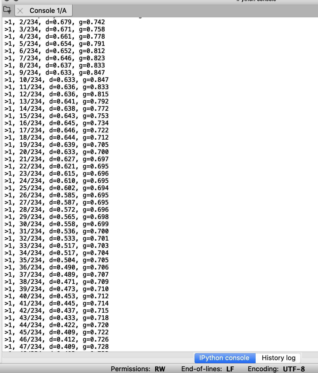
# summarize loss on this batch
print('>%d, %d/%d, d=%.3f, g=%.3f' % (i+1, j+1, bat_per_epo, d_loss, g_loss))
There it is guys! That’s the showdown we’ve all been waiting for! The generator will try to synthesize images to ‘bypass’ or ‘fool’ the discriminator and the discriminator will try to foil the attempts of the generator, indirectly causing the generator to step his game up and create better fakes to finally bypass the discriminator.
Does it succeed in our case?
We’ll find out.
On running the code, we get the following output:
The only thing remaining now is evaluation.
VII. Evaluation
Generally, there are no objective ways to evaluate the performance of a GAN model.
We cannot calculate this objective error score for generated images.
Instead, images must be subjectively evaluated for quality by a human operator. This means that we cannot know when to stop training without looking at examples of generated images. In turn, the adversarial nature of the training process means that the generator is changing after every batch, meaning that once “good enough” images can be generated, the subjective quality of the images may then begin to vary, improve, or even degrade with subsequent updates.
There are three ways to handle this complex training situation.
- Periodically evaluate the classification accuracy of the discriminator on real and fake images.
- Periodically generate many images and save them to file for subjective review.
- Periodically save the generator model.
All three of these actions can be performed at the same time for a given training epoch, such as every five or 10 training epochs. The result will be a saved generator model for which we have a way of subjectively assessing the quality of its output and objectively knowing how well the discriminator was fooled at the time the model was saved. Training the GAN over many epochs, such as hundreds or thousands of epochs, will result in many snapshots of the model that can be inspected and from which specific outputs and models can be cherry-picked for later use.
First, we can define a function called summarize_performance() function that will summarize the performance of the discriminator model. It does this by retrieving a sample of real MNIST images, as well as generating the same number of fake MNIST images with the generator model, then evaluating the classification accuracy of the discriminator model on each sample and reporting these scores. Next, we can update the summarize_performance() function to both save the model and to create and save a plot generated examples. As we are evaluating the discriminator on 100 generated MNIST images, we can plot all 100 images as a 10 by 10 grid.
# evaluate the discriminator, plot generated images, save generator model
def summarize_performance(epoch, g_model, d_model, dataset, latent_dim, n_samples=100):
	# prepare real samples
	X_real, y_real = generate_real_samples(dataset, n_samples)
	# evaluate discriminator on real examples
	_, acc_real = d_model.evaluate(X_real, y_real, verbose=0)
	# prepare fake examples
	x_fake, y_fake = generate_fake_samples(g_model, latent_dim, n_samples)
	# evaluate discriminator on fake examples
	_, acc_fake = d_model.evaluate(x_fake, y_fake, verbose=0)
	# summarize discriminator performance
	print('>Accuracy real: %.0f%%, fake: %.0f%%' % (acc_real*100, acc_fake*100))
	# save plot
	save_plot(x_fake, epoch)
	# save the generator model tile file
	filename = 'generator_model_%03d.h5' % (epoch + 1)
	g_model.save(filename)
We put this function we’ve written in the def_train() function for evaluation as follows:
# train the generator and discriminator
def train(g_model, d_model, gan_model, dataset, latent_dim, n_epochs=100, n_batch=256):
	bat_per_epo = int(dataset.shape[0] / n_batch)
	half_batch = int(n_batch / 2)
	# manually enumerate epochs
	for i in range(n_epochs):
		# enumerate batches over the training set
		for j in range(bat_per_epo):
			# get randomly selected 'real' samples
			X_real, y_real = generate_real_samples(dataset, half_batch)
			# generate 'fake' examples
			X_fake, y_fake = generate_fake_samples(g_model, latent_dim, half_batch)
			# create training set for the discriminator
			X, y = vstack((X_real, X_fake)), vstack((y_real, y_fake))
			# update discriminator model weights
			d_loss, _ = d_model.train_on_batch(X, y)
			# prepare points in latent space as input for the generator
			X_gan = generate_latent_points(latent_dim, n_batch)
			# create inverted labels for the fake samples
			y_gan = ones((n_batch, 1))
			# update the generator via the discriminator's error
			g_loss = gan_model.train_on_batch(X_gan, y_gan)
			# summarize loss on this batch
			print('>%d, %d/%d, d=%.3f, g=%.3f' % (i+1, j+1, bat_per_epo, d_loss, g_loss))
		# evaluate the model performance, sometimes
		if (i+1) % 10 == 0:
			summarize_performance(i, g_model, d_model, dataset, latent_dim)
In the last 3 lines of the above code, we’ve inserted the summarize_performance method.
VIII. Conclusions & Results
On running the entire code as a whole, you should see that the GAN begins to train. The model performance is reported every batch, including the loss of both the discriminative (d) and generative (g) models. The generator is evaluated every 20 epochs, resulting in 10 evaluations, 10 plots of generated images, and 10 saved models.
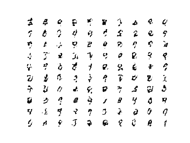
For our run, the results after 10 epochs were found to be low quality, although we can see that the generator has learned to generate centered figures in white on a back background
After 20 or 30 more epochs, the model begins to generate very plausible MNIST figures,
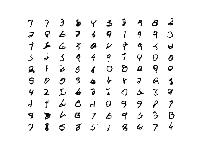
The generated images after 100 epochs are not greatly different, but we can detect less blocky-ness in the curves.
It should be noted that the performance of a GAN may deteriorate over the epochs. It is not necessary that the performance obtained at the 100th epoch will be better or even as good as the performance obtained at the 40th epoch. Therefore, it is always a good practice to use the functions provided in this blog whenever training a GAN so you can visualize what actually is the best performance for your particular application.
Once a final generator model is selected, it can be used in a standalone manner for your application.
This involves first loading the model from a file, then using it to generate images. The generation of each image requires a point in the latent space as input.
The complete example of loading the saved model and generating images is listed below. In this case, we will use the model saved after 100 training epochs, but the model saved after 40 or 50 epochs would work just as well.
# generate points in latent space as input for the generator
def generate_latent_points(latent_dim, n_samples):
	# generate points in the latent space
	x_input = randn(latent_dim * n_samples)
	# reshape into a batch of inputs for the network
	x_input = x_input.reshape(n_samples, latent_dim)
	return x_input

# create and save a plot of generated images (reversed grayscale)
def save_plot(examples, n):
	# plot images
	for i in range(n * n):
		# define subplot
		pyplot.subplot(n, n, 1 + i)
		# turn off axis
		pyplot.axis('off')
		# plot raw pixel data
		pyplot.imshow(examples[i, :, :, 0], cmap='gray_r')
	pyplot.show()

# load model
model = load_model('generator_model_100.h5')
# generate images
latent_points = generate_latent_points(100, 25)
# generate images
X = model.predict(latent_points)
# plot the result
save_plot(X, 5)
Running the example first loads the model samples 25 random points in the latent space, generates 25 images, then plots the results as a single image.
We can see that most of the images are plausible, or plausible pieces of handwritten digits.

This concludes the complete code example for GANs. In the subsequent blogs, we’ll take up the more advanced variations in GANs that have come up in the literature over the past few years. Specifically, we’ll be looking at the pix2pix GAN used for image translation tasks in the next blog.
Be sure to tune in you do not want to miss this! Not sure if the showdown lived up to its expectation but we’re sure it enticed the readers. GANs are, after all, the bleeding edge in AI.
More from the Series:
- An Introduction to Generative Adversarial Networks- Part 1
- pix2pix GAN: Bleeding Edge in AI for Computer Vision- Part 3
- CycleGAN: Taking It Higher- Part 4
- The Grand Finale: Applications of GANs- Part 5
Looking for Online Learning? Here’s what you can choose from!
- Deep Learning & Neural Networks Using Python & Keras For Dummies
- Learn Machine Learning By Building Projects
- Machine Learning With TensorFlow The Practical Guide
- Deep Learning & Neural Networks Python Keras For Dummies
- Mathematical Foundation For Machine Learning and AI
- Advanced Artificial Intelligence & Machine Learning (E-Degree)
References
[1] Generative Adversarial Networks, 2014
Ian J. Goodfellow, Jean Pouget-Abadie, Mehdi Mirza, Bing Xu, David Warde-Farley, Sherjil Ozair, Aaron Courville, Yoshua Bengio
[2] Deep Boltzmann Machines, 2013
Ruslan Salakhutdinov, Geoffrey Hinton
[3] An Introduction to Restricted Boltzmann Machines, 2012
Asja FischerChristian Igel
[4]How to Develop a GAN for Generating MNIST Handwritten Digits
Jason Brownlee
[5] Improved Techniques for Training GANs
https://arxiv.org/abs/1606.03498?source=post_page—–b665bbae3317———————-


")


